
7.1 Capacitors
Capacitors are circuit elements that store energy in an electric field between two charged surfaces, analogous to the way the potential energy of a lifted mass represents energy stored in a gravitational field. A capacitor is constructed from two conducting plates separated from each other by a layer of dielectric material (dielectric refers to insulating material, such as air, plastic, teflon, etc…) as illustrated below. When the terminals of a battery are connected to the conducting plates, charges are deposited on the plates, positive charges on the plate connected to the battery’s + terminal and negative charges on the plate connected to the battery’s – terminal.
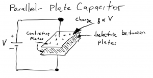
The charge on the plates (+q on the upper plate, -q on the lower plate in the diagram) is proportional to the applied voltage, q∝V. The constant of proportionality is the capacitance, C, having units of volts/coulomb or farads (F). This,
(1) 
In general, voltage is a function of time, and we have
(2) 
Capacitor values range from tiny pF (10-12 F) to several thousand F (kF, called “supercaps”). We will work with capacitors in the lab experiments of this book having values of 0.1 μF and 10 μF. Most of our concern, and discussion, will be with the use of capacitors in circuits, so we will not be overly concerned with the physics of capacitors or with their construction. Instead, we will be working with circuit-level characterization such as the V-I relationship and with expressions of power and energy associated with capacitors. But it is useful to briefly digress and look at common capacitor values and construction.
The capacitance of parallel-plate capacitor such as that shown above is C=εA/d where A is the area of the conducting plate (lenght x width), d is the separation between the plates, and ε is the permittivity of the medium between the plates. For free-space, ε=8.85×10⁻¹² F/m, and for other media, ε is this value multiplied by the dielectric constant of the medium, with 2-4 being typical values. Thus, a capacitor made from 10 cm x 10 cm plates separated by 1μm (10-6 m) with free space between the plates, has a capacitance of 8.854×10-12 x .1 x .1/1×10-6 = 88.5 x 10⁻⁹ F or 88.5 nF. There exist many techniques for manufacturing different types of capacitor.
Voltage-current relationship for a capacitor. Current is the time derivative of charge,  . Charge is given by equation Xx, and since C is a constant (no time variation), we have
(3) 
Often we will omit the time dependence, as it is implied by the use of lower-case variable i and v:
(4) 
Example: A voltage v(t), shown below, is connected across a 1 nF capacitor. Determine and sketch the current as a function of time.
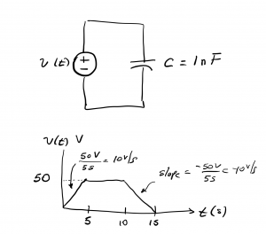
Solution:
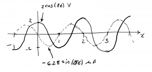
Example: A voltage v(t) = 2cos(πt) is applied across a 1 μF capacitor. Sketch v(t) and i(t) as a function of time.
Solution:
Capacitor voltage as a function of current. We now develop the v(t) vs. i(t) relationship. We begin by recalling q(t)=Cv(t), from which we have  . We can determine q(t) by recalling that current is the time-derivative of charge,
(5) 
multiplying both sides of this equation by  and integrating from -∞ to t, we have
(6) 
canceling dt and changing the limits of integration on the right side of the equation gives
(7) 
We can change the lower integration limit from -∞ to whatever time we start considering the circuit, to
(8) 
which results in
(9) 
giving the charge as a function of time in terms of the integral of the current, plus any initial charge at time t_o:
(10) 
since v(t)=q(t)/C. we have
(11) 
the term q(t_o)/C, which has units of coulombs/farad or coulombs/(volt/coulomb) = volts, represents the initial voltage on the capacitor at time t=t_o. We therefore re-write this equation in terms of v_o:
(12) 
We see that the voltage on the capacitor at time t, is any initial voltage, v_o, plus the increase in voltage due to the action of current in depositing charge on the capacitor plates. (Re-watch the demo video at the beginning of this chapter.)
Example: The current through a capacitor is given by XXXX. Determine and sketch the voltage versus time, v(t).
Equivalent capacitance: capacitors in series. Just as we are able to replace networks of resistors with equivalent resistors but exploiting series and parallel combinations, we can also do this with capacitors. First, we consider N capacitors connected in series and we work to determine the value of the equivalent capacitance, Ceq.

We approach this problem by considering two circuits shown, and we want equivalent v(t) vs i(t) relationships. To simplify the analysis, we assume that all capacitors initially have zero voltage.
The capacitor on the right has the v(t) vs i(t) relationship:
(13) 

For the series connection of capacitors on the left, we perform KVL to obtain
(14) 
We next write the capacitor voltages in terms of current i(t), noting that i(t) is the current through each of the series capacitors on the left.
(15) 
the integral is common to all terms and can be factored, resulting in
(16) ![\begin{equation*} v(t)=[\frac{1}{C_1}+\frac{1}{C_2}+...+\frac{1}{C_N}]\int_0^t i(t)dt \end{equation*}](http://openbooks.library.umass.edu/funee/wp-content/ql-cache/quicklatex.com-6502c057d65857813aeb3caa5814f3ed_l3.png "Rendered by QuickLaTeX.com")
equating equations XX and XX, we see that
(17) 
from which we have
(18) 
Note that a set of identical capacitors connected in series has lower capacitance than a single capacitor alone. Why? Recall that capacitance is the ratio of voltage to charge. When a set of capacitors is wired in series, the overall voltage drop is shared among the set of capacitors (ie, each has a fraction of the overall voltage); the current through each capacitor, and hence the rate at which charge is deposited, is the same, so the capacitance of each is lower than the capacitance of a single capacitor.
Capacitors in parallel. We now consider equivalent capacitance when a set of N capacitors are connected in parallel as shown.
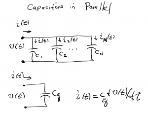
The i(t) vs v(t) relationship for the equivalent capacitance is given by
(19) 
To develop the i(t) vs v(t) relationship for the parallel set of capacitors, we apply KCL to the top node:
(20) 
since the voltage across each of the parallel capacitors is v(t), we can write
(21) 
factoring the common v(t) term results in
(22) ![\begin{equation*} i(t) =[C_{1} + C_{2} +...+C_{N}]\frac{dv(t)}{dt}\end{equation*}](http://openbooks.library.umass.edu/funee/wp-content/ql-cache/quicklatex.com-d82865281493c8ddd938b7f1a96a4f9e_l3.png "Rendered by QuickLaTeX.com")
comparing equations XX and YY, we conclude
(23) 
Note that capacitors connected in parallel, combine arithmetically like resistors in series: they add. That is, capacitance increases when multiple capacitors are combined in parallel. Why? Capacitance is the ratio of charge to voltage, so larger charge for a given voltage represents larger capacitance. When a set of capacitors is connected in parallel, they all have the same voltage, yet they each independently draw current from the voltage source. Consequently, they each build up charge, and the result has higher charge than a single capacitor by itself. For this reason, identical capacitors wired in parallel have higher capacitance than a single capacitor having the same individual capacitance.
Examples: determine the capacitance of two identical caps in parallel and 2 in series. Develop an equations like for resistors and compare.
