2.8 Power and energy in resistive circuits

David J. McLaughlin

2.8 Power and energy in resistive circuits

We now consider the power and energy absorbed by resistors and supplied by sources in more detail. Recall that a voltage drop (a decrease in electric potential) across a circuit element in the direction of positive current flow represents energy absorbed. This is the case when current moves through a resistor. A voltage rise (an increase in electric potential) across a circuit element in the direction of positive current flow represents energy being supplied by the circuit element. This is the case when a battery supplies power to a circuit. In either case, energy is being transferred (such as being converted to heat or being supplied to the circuit) at a rate of

(1) $\begin{equation*} p(t)=v(t) \cdot i(t) \end{equation*}$

which has units of watts or $\frac{Joules}{second}$ . To better understand eq (1), we can rewrite the equation in terms of the unit dimensions for power, voltage and current

(2) $\begin{equation*} \frac{J}{s} = \frac{J}{C}\cdot \frac{C}{s} \end{equation*}$

For a resistor, Ohm’s law equations $v(t)=i(t)R$ and $i(t)=\frac{v(t)}{R}$ can be used in eq (1) to obtain

(3) $\begin{equation*} p(t)=\frac{v(t) ^{2}}{R} \end{equation*}$

and

(4) $\begin{equation*} p(t)=i(t)^{2}R \end{equation*}$

respectively. Equations (1), (3) and (4) are all useful for for determining the power absorbed by a resistor.

Energy supplied or absorbed. Since power is the rate of transfer of energy ( $\frac{J}{s}$ ) The total energy transferred over a time interval $\tau$ seconds long from $t_{0}$ to $t_{0}+\tau$ is given by

(5) $\begin{equation*} E = \int_{t_{0}}^{t_{0}+\tau} p(t) dt \end{equation*}$

Note that we have explicitly noted the time dependence for voltage $v(t)$ , current $i(t)$ and power $p(t)$ in the expressions discussed above. This makes it easier to remember that AC waveforms vary as functions of time. Below, we consider DC and AC circuits and power calculations, and we will find, not surprisingly, that $p(t)$ is constant for DC circuits while $p(t)$ varies with time for AC circuits. Looking ahead, we will develop expressions for computing average power when $p(t)$ fluctuates with time, and we will find that, for circuits comprised of resistors and sources, the average power is conveniently related to the RMS values of voltage and current.

DC circuit example. Consider the circuit shown in figure 2.70 where $v(t)$ is a DC voltage given by

(6) $\begin{equation*} v(t)=V_{DC} \end{equation*}$

Figure 2.70 Resistor circuit with a DC voltage source

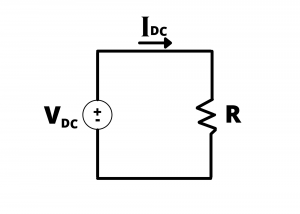
The power absorbed by the resistor is, using (3)

(7) $\begin{equation*} p(t)=\frac{V_{DC}^2}{R}\end{equation*}$

and the amount of energy absorbed by the resistor over the time interval from $0$ to $\tau$ is

(8) $\begin{equation*} E = \int_{0}^{\tau} p(t) dt= \int_{0}^{10} \frac{V_{DC}^2}{R} dt =\frac{V_{DC}^2\tau}{R}\end{equation*}$

Examples

Example: If $V_{DC}$ in Figure 2.70 were $6V$ and $R=100\Omega$ how much energy would be absorbed by the resistor in 10 seconds? 100 seconds? for all time?

Solution: By eq (8), $E = \frac{V_{DC}^2\tau}{R}=\frac{6^2 10}{100}=3.6J$ for $\tau=10s$ . For $\tau=100 s$ $E=36J$ . For all time, $E$ would be infinite. This, of course, is not practical, but neither is it practical to have a voltage source that lasts for all of time.

Example: If $V_{DC}$ in Figure 2.70 were $6V$ and $R=100\Omega$ how long would it take until all the energy in the batteries was depleted if the $6V$ power supply was comprised of four fresh AA batteries wired in series, each containing 10kJ of energy when new.

Solution: The total energy from the batteries is $4 \cdot 10k J= 40k J$ . From eq (7) the circuit is consuming energy at a rate $\frac{V_{DC}^2}{R}=\frac{6^2}{100}=0.36 \frac{J}{s}$ . The battery’s energy will be consumed in $\frac{40\cdot 10^{3}}{0.36} = 1.1\cdot 10^{5} s$ or $30.9$ hours (hr).

AC circuit example. We now consider the power and energy associated with resistive circuits driven by AC sources. Consider the circuit shown in figure 2.70 where $v(t)$ is an AC voltage source given by

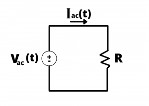
(9) $\begin{equation*} v(t)=v_{ac}(t)=V_{m}\cos(\frac{2\pi t}{T}) \end{equation*}$

Figure 2.71 Resistor circuit with an AC voltage source

The current is given by

(10) $\begin{equation*} i(t)=i_{ac}(t)=\frac{v_{ac}}{R}=\frac{V_{m}}{R}\cos(\frac{2\pi t}{T}) \end{equation*}$

The instantaneous power absorbed by the resistor is, using (3)

(11) $\begin{equation*} p(t)=\frac{v^{2}_{ac}}{R}=\frac{V_{m}^{2}}{R} \cos^{2}(\frac{2\pi t}{T})\end{equation*}$

The instantaneous waveforms for $v(t)$ , $i(t)$ , and $p(t)$ are plotted in figure 2.71 for time from $t=0$ to $t=3.5T$ seconds. Note how the voltage oscillates between peak-to-peak values $V_{m}$ to $-V_{m}$ over time, while current simultaneously oscillates between peak-to-peak values $\frac{V_{m}}{R}$ to $-\frac{V_{m}}{R}$ amps. The RMS value for the voltage,

(12) $\begin{equation*} V_{rms}=\sqrt{\frac{1}{T}\int_{0}^{T} v^{2}(t)dt}=\frac{V_{m}}{\sqrt 2} = 0.707V_{m} \end{equation*}$

is shown as a dashed line in the $v(t)$ plot. Likewise, the RMS value for the current, which is $\frac{1}{\sqrt{2}}$ or $0.707$ times the peak value, is shown as a dashed line on the $i(t)$ plot.

Figure 2.72 Instantaneous voltage, current, and power versus time. Dashed lines are RMS voltage (top), RMS current (middle) and Average power (bottom)

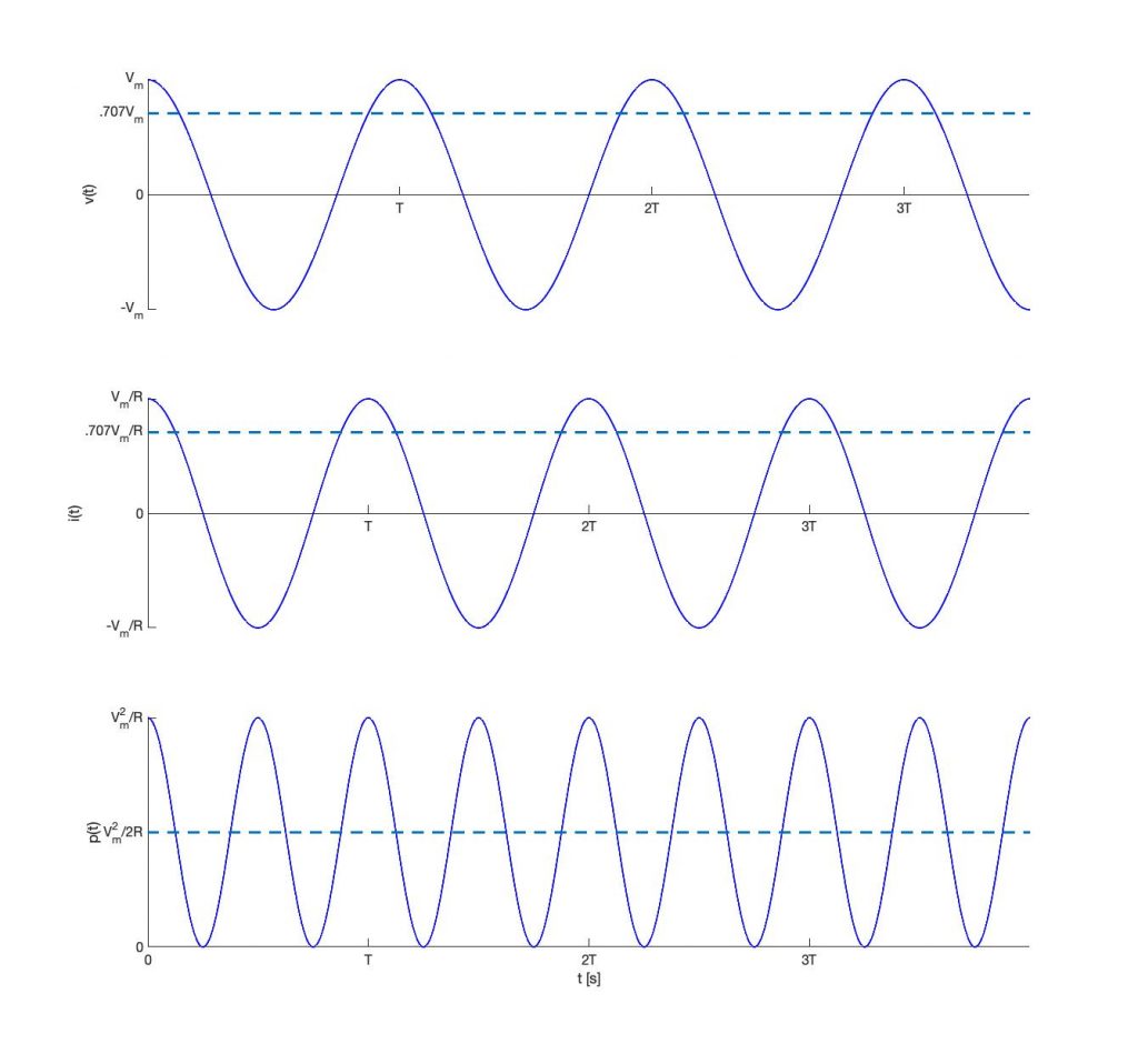
Owing to the sinusoidal character of the voltage and current waveforms, the instantaneous power also has a sinusoidal character. The instantaneous power $p(t)$ has the shape of a raised cosine oscillating at twice the frequency of $v_{ac}(t)$ ; this is evident when we apply the trigonometric identity:

(13) $\begin{equation*} \cos^{2}(x)= \frac{1}{2} (1 + \cos(2x)) \end{equation*}$

to eq (11) to give

(14) $\begin{equation*} p(t)=\frac{V^{2}_{m}}{2R}[1+\cos(4\pi t)] \end{equation*}$

The average power, computed as

(15) $\begin{equation*} P_{AVE}=\frac{1}{T} \int_{0}^{T} p(t) dt = \frac{1}{T} \int_{0}^{T} \frac{V^{2}_{m}}{2R}[1+\cos(4\pi t)] dt = \frac{V^{2}_{m}}{2R}\end{equation*}$

is plotted as a dashed line on the $p(t)$ plot of figure 2.71.

Note that the product of the RMS voltage and RMS current is equal to the average power:

(16) $\begin{equation*} P_{AVE}=V_{rms} I_{rms} = \frac{V_{m}}{\sqrt{2}} \frac{I_{m}}{\sqrt{2}} = \frac{V_{m}}{\sqrt{2}} \frac{V_{m}}{\sqrt{2}R}= \frac{V^{2}_{m}}{2R}= \frac{V^{2}_{rms}}{R} \end{equation*}$

which gives

(17) $\begin{equation*} P_{AVE}= \frac{V^{2}_{m}}{2R} =\frac{V^{2}_{rms}}{R} \end{equation*}$

Recall that power is the rate at which energy is absorbed. The total amount of energy absorbed by resistor $R$ between $t=0$ and $t=\tau$ seconds is, from eq(5)

(18) $\begin{equation*} E =\frac{1}{T} \int_{0}^{\tau} p(t) dt = \int_{0}^{\tau} \frac{V^{2}_{m}}{2R}[1+\cos(4\pi t)] dt \end{equation*}$

If $\tau$ is a multiple of $T$ then the $\cos(4\pi t)$ integrand of eq (19) evaluates to zero, and we have

(19) $\begin{equation*} E =\frac{V^{2}_{m}\tau}{2R}= \frac{V^{2}_{rms}\tau}{R}\end{equation*}$

Note the use of $T$ and $\tau$ in these equations. $T$ refers to the repetition period of the periodic waveforms under consideration. All of the structure of a periodic waveform is represented in a time interval $T$ seconds long, and we can actually carry out integrals over any duration $T$ seconds wide, although we are using the internal from $t=0$ to $t=T$ seconds here. The variable $\tau$ represents the duration over which we are calculating energy absorbed, and this need not be related to T. As an example, we might want to determine how much energy is absorbed by a household appliance over a day. Since household electricity in the USA oscillates at 60 Hz, calculations would use $T=\frac{1}{60} s$ , while $\tau = 3600 \cdot 24= 86400$ is the number of seconds in a day.

Average power for periodic waveforms. The results given above relating the average power and the total energy over a finite time interval to the RMS voltage have been derived specifically for the case of a sinusoidal waveform, but these results are valid for any periodic waveform. This is apparent when we write the equation for average power:

(20) $\begin{equation*} P_{AVE}=\frac{1}{T} \int_{0}^{T} p(t) dt = \frac{1}{T} \int_{0}^{T} v(t)i(t)dt\end{equation*}$

for a resistor, $i(t)=\frac{v(t)}{R}$ and equation (20) can be written as

(21) $\begin{equation*} P_{AVE}=\frac{1}{T} \int_{0}^{T} \frac{v^{2}(t)}{R}dt=\frac{1}{R} \cdot\frac{1}{T} \int_{0}^{T} v^{2}(t)dt\end{equation*}$

when $\frac{1}{R}$ is removed from the integral, and when we recall the definition previously given for the RMS voltage:

(22) $\begin{equation*} V_{rms}=\sqrt{\frac{1}{T} \int_{0}^{T} v^{2}(t)dt\end{equation*}$

we have the result

(23) $\begin{equation*} P_{AVE}=\frac{V^{2}_{rms}}{R} \end{equation*}$

License

Icon for the Creative Commons Attribution 4.0 International License

Applied Electrical Engineering Fundamentals by David J. McLaughlin is licensed under a Creative Commons Attribution 4.0 International License, except where otherwise noted.

License

Share This Book