
2.5 AC and DC waveforms, average and RMS values
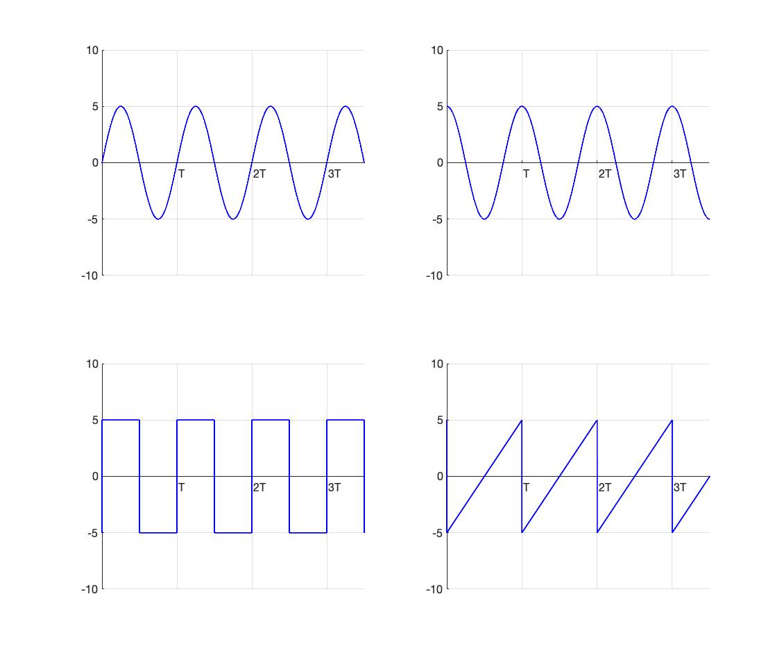
AC, DC, and mixed waveforms. Figure 2.42 shows a set of periodic time-varying AC waveforms plotted as functions of time. The period in each case is T seconds, meaning that each waveform repeats every integral multiple of T seconds, and we can write
(1) 
We are going to determine the average value of each of these waveforms and we will find it equal to zero in each case. This is a characteristic of all AC waveforms. (Before proceeding to compute average values analytically, we might note that, in the case of these particular waveforms, we can see by inspection that they all have zero-average. Looking at the curves and noting that the area under each curve for positive excursions of the waveforms, ie, when  is equal to the area under the curve for negative excursions, ie, when
  , we can deduce that they all have an average value of zero.)
We determine the average value of these waveforms analytically, by computing
(2) 
Note that the integral can be carried out over any time span T seconds in duration.
The first waveform is characterized by
(3) 
and the average is
(4) 
(5) 
(6) ![\begin{equation*} =\frac{5}{2\pi} [ \cos(2\pi) - \cos(0)] \end{equation*}](http://openbooks.library.umass.edu/funee/wp-content/ql-cache/quicklatex.com-8f05a524c355965b6e064dd0c90969d3_l3.png "Rendered by QuickLaTeX.com")
(7) 
The cosine waveform in the upper-right of Figure 2.30 has the expression
(8) 
Likewise, the average value of the cosine waveform (upper right) is also zero.
For the square wave in the lower left of figure 2.42, we note that the waveform has value  in the interval between
  and
and  and value
  in the interval between and
  . The average is then given as
(9) ![\begin{equation*} V_{AVE}= \frac{1}{T} [\int_{0} ^{\frac{T}{2}} 5 dt + \int_{\frac{T}{2}} ^{T} -5 dt]\end{equation*}](http://openbooks.library.umass.edu/funee/wp-content/ql-cache/quicklatex.com-02d59b67df45a4ba1ff20def0f064a83_l3.png "Rendered by QuickLaTeX.com")
(10) ![\begin{equation*} = \frac{1}{T} [\frac{5T}{2} - \frac{5T}{2}]\end{equation*}](http://openbooks.library.umass.edu/funee/wp-content/ql-cache/quicklatex.com-33974ea6c64241f48da6331cc0a59d9f_l3.png "Rendered by QuickLaTeX.com")
(11) 
The sawtooth waveform can be characterized in the interval between and by
(12) 
so that
(13) 
(14) ![\begin{equation*} = \frac{1}{T} [ \frac{10t^{2}}{2T}|_{0}^{T} - 5t |_{0}^{T} ] \end{equation*}](http://openbooks.library.umass.edu/funee/wp-content/ql-cache/quicklatex.com-2f05f338df1f7a5f236593399a2fb4b4_l3.png "Rendered by QuickLaTeX.com")
(15) ![\begin{equation*} = \frac{1}{T} [ \frac{10T}{2} - 5T] \end{equation*}](http://openbooks.library.umass.edu/funee/wp-content/ql-cache/quicklatex.com-f0e914d1a4851ae49d35bc930a4d195e_l3.png "Rendered by QuickLaTeX.com")
(16) 
We thus see that average value of each of the four waveforms plotted in figure 2.42 is zero. This is the case with any AC waveform
Mixed AC and DC waveforms. Now consider the periodic waveforms shown in figure 2.43. Are these AC waveforms? If these waveforms represented current sources, would they represent currents that alternate direction over time? Clearly, they are not DC waveforms, constant and ever-fixed, not varying with time. The waveforms shown in the upper left and the lower right and lower left are all positive-valued waveforms; they fluctuate over time, but they do not achieve negative values. If they represented currents, those currents would not change direction over time as would be the case for an AC current. The waveform shown in the upper-right goes slightly negative for a small portion of the repeat period; if this were a current, it would reverse direction for a small portion of the repeat period. These waveforms are all composites, or superpositions, of AC and DC waveforms.
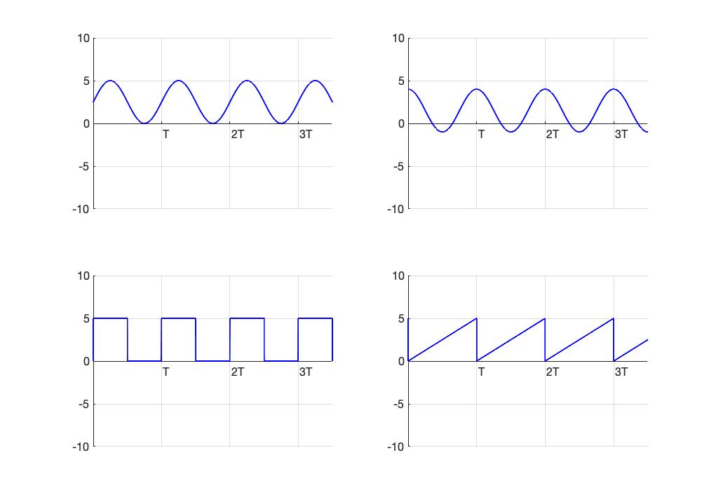
The waveform in the upper-left is characterized by the expression:
(17) 
This “raised sine” is a combination of an AC component,  and a DC component,
  . If we computed the average value of this waveform, we would find it equal to the DC component,
(18) 
This analysis applies to all the waveforms shown in figure 2.43 and allows us to state the observation that the average of any periodic waveform is equal to the DC component of that waveform. This is actually what is measured when a multimeter is configured to perform a DC voltage or current measurement.
The average of any periodic waveform is equal to its DC component.
(19) 
A DC measurement on a multimeter is the average value of the signal.
Examples
Example: Determine the DC component, or the DC value, of the raised cosine in the upper-right of figure 2.31 if the waveform is given by 
Solution: The average value of the waveform is given by
(20) 
Example: Determine the DC component of the square wave shown in the lower left of figure 2.31.
Solution: The waveform has value over the interval from to and  over the interval from to . The average value is
  .
.
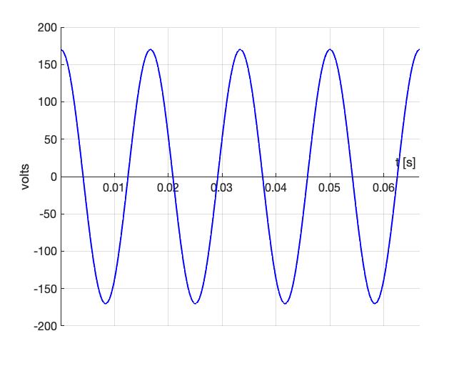
RMS or effective value. We now know that a DC waveform can be characterized by a single number. Likewise, the DC component of a waveform comprised of an AC and a DC component can be characterized by the average value of that waveform. Can we characterize an AC waveform with a single number? Consider the instantaneous voltage versus time for an AC electrical outlet that we discussed earlier in this chapter. The waveform is given by the expression
(21) 
and plotted in figure 2.44. We see that the voltage oscillates between a peak or maximum positive value of  and a peak negative value of
  .
.
 plotted versus time
A multimeter measurement of the AC voltage from an outlet is shown below.
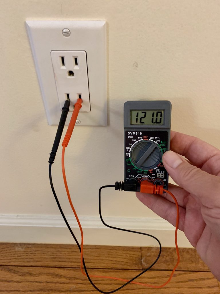
When set to read AC voltage, the meter reading is 121 Volts AC. The meter is providing only a single value that effectively represents the intensity of the oscillating AC waveform of figure 2.44. This “effective voltage” is the RMS or root-mean-square value of the AC waveform. The RMS voltage is given by the equation:
(22) 
As specified by its name, this expression computes the square root of the mean (average) of the square of the waveform. This calculation gives a measure of the intensity of a waveform and provides a means to characterize waveform intensity even for waveforms having a mean (or average) value of zero. The RMS value for the electrical wall outlet characterized by eq. (21) is:
(23) ![\begin{equation*} V_{rms}= \sqrt{ \frac{1}{\frac{1}{60}} \int_{0} ^{\frac{1}{60}} [170\cos(120\pi t)]^{2} dt } \end{equation*}](http://openbooks.library.umass.edu/funee/wp-content/ql-cache/quicklatex.com-ce66a1da9e5dd538142526d76f906c5f_l3.png "Rendered by QuickLaTeX.com")
where  in the integral is given the value
  since electrical wall outlet voltages in the USA oscillate at a frequency
  . Making use of the trigonometric identity
(24) ![\begin{equation*} \cos^{2}(x)= \frac{1}{2} [\cos(2x)+1] \end{equation*}](http://openbooks.library.umass.edu/funee/wp-content/ql-cache/quicklatex.com-7e8ee421e67db72616153d501525619b_l3.png "Rendered by QuickLaTeX.com")
we have
(25) ![\begin{equation*} V_{rms} = \sqrt{ 60 \frac{170^{2}}{2} \int_{0} ^{\frac{1}{60}} [\cos(240\pi t) +1] dt } \end{equation*}](http://openbooks.library.umass.edu/funee/wp-content/ql-cache/quicklatex.com-318c54f503b23f275660a343d4e55a95_l3.png "Rendered by QuickLaTeX.com")
(26) 
which is close to the RMS voltage read by the multimeter. The nominal voltage for a wall outlet in the USA is 120  but it can range between 114 and 126 .
The RMS value for any sinusoidal signal  having peak amplitude
  is given by
(27) ![\begin{equation*} V_{rms}= \sqrt{ \frac{1}{T} \int_{0} ^{T} [V_{m}\cos(\frac{2\pi t}{T})]^{2} dt } \end{equation*}](http://openbooks.library.umass.edu/funee/wp-content/ql-cache/quicklatex.com-64a4cf7b6e243568cf7a16bcf79b08e6_l3.png "Rendered by QuickLaTeX.com")
(28) 
making use of the trigonometric identity of eq (24),
(29) ![\begin{equation*} V_{rms} = \sqrt{ \frac{1}{T} \int_{0} ^{T} \frac{V^{2}_{m}}{2}[1+\cos(\frac{4\pi t}{T})] dt } \end{equation*}](http://openbooks.library.umass.edu/funee/wp-content/ql-cache/quicklatex.com-370403b09a14746cbb7fb14c838f79c9_l3.png "Rendered by QuickLaTeX.com")
(30) 
since the second integral evaluates to zero, we have
(31) 
(32) 
This result applies for any sinusoidal waveform.
The RMS value is not used only for sinusoids. Equation (22) can be used to determine the RMS value for any periodic waveform.
Examples
Example: Determine the RMS value for the raised sawtooth wave in the lower-right of Figure 2.43.
Solution: During the period from to the waveform is given by  . The RMS value is computed as
(33) 
Example: Determine the RMS value for the waveform 
Solution: This waveform obviously has a DC component and an AC component. The RMS value is, from eq (22),
(34) ![\begin{equation*} V_{rms} = \sqrt{ \frac{1}{T} \int_{0} ^{T} [A+B\cos(\frac{2\pi t}{T})]^{2} dt} \end{equation*}](http://openbooks.library.umass.edu/funee/wp-content/ql-cache/quicklatex.com-bd914ed28619be5f834fe29edde77a9e_l3.png "Rendered by QuickLaTeX.com")
(35) ![\begin{equation*} = \sqrt{ \frac{1}{T} \int_{0} ^{T} [A^{2}+2AB\cos(\frac{2\pi t}{T}) +B^{2}\cos^{2}(\frac{2\pi t}{T}) ]dt }\end{equation*}](http://openbooks.library.umass.edu/funee/wp-content/ql-cache/quicklatex.com-a4dda898f6576a56c70b25a2c9f39c39_l3.png "Rendered by QuickLaTeX.com")
(36) ![\begin{equation*} = \sqrt{ \frac{1}{T} \int_{0} ^{T} [A^{2}+2AB\cos(\frac{2\pi t}{T}) +\frac{B^{2}}{2} [1+\cos(\frac{4\pi t}{T})] ]dt }\end{equation*}](http://openbooks.library.umass.edu/funee/wp-content/ql-cache/quicklatex.com-921278836367b2660e59e737793a2e62_l3.png "Rendered by QuickLaTeX.com")
since all the terms involving  will integrate to zero, we have
(37) ![\begin{equation*} = \sqrt{ \frac{1}{T} \int_{0} ^{T} [A^{2}+\frac{B^{2}}{2} ]dt }\end{equation*}](http://openbooks.library.umass.edu/funee/wp-content/ql-cache/quicklatex.com-366e4619f3c999300db63da967b97b48_l3.png "Rendered by QuickLaTeX.com")
(38) 
We could have written the waveform for the previous example problem as
(39) 
where  and
and  .
.
From our previous discussion, we know the RMS value of the ac component is  . The result given in eq (38) can be written as
(40) 
.
While this result happens to have been derived specifically for a sinusoidal AC signal. the result given in eq(40) is applicable to any AC waveform.
The rms value for any periodic waveform having period is computed as
(41) 
This is the value read by an AC voltmeter or AC ammeter.
For any sinusoidal waveform  the RMS value is
  .
.
For any waveform comprised of a DC component and an AC component,  , the rms value is given by
  where
where  is the RMS value of the AC component of the waveform,
  .
.
