2.2 First Circuit

David J. McLaughlin

2.2 First Circuit

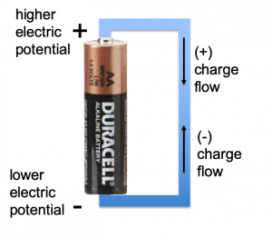
Consider an alkaline dry-cell battery, such as the 1.5 volt AA (or AAA) battery that powers a portable calculator or TV remote. The inside of the battery contains electrochemical cells situated between a pair of electrodes, which serve as the battery terminals. Chemical reactions taking place within the cells deposit a supply of charges on the electrodes, with positive charges on the positive electrode and negative charges on the negative electrode. The charge imbalance between the electrodes causes an electric potential difference to be maintained between the battery terminals. The positive terminal $(+)$ has an electric potential $1.5 \frac{J}{C}$ higher than the negative $(-)$ terminal. We refer to this electric potential difference as voltage difference such that the positive terminal of the battery is $1.5$ volts ( $V$ ) higher than the negative terminal. Conversely, the negative terminal has an electric potential $1.5 V$ lower than the positive terminal. It is the difference in electric potential (or the difference in voltage) between the terminals that matters in terms of forcing charges to move around in a circuit, as we shall see below. We usually refer to the voltage difference as the voltage across the battery; that is, the voltage across the battery is $1.5 V$ , since there is a $1.5$ volt difference between the $+$ and $-$ terminals of the battery. Later in this text, we will use the terms voltage rise and voltage drop to refer to the way voltages increase across devices such as batteries (energy sources) and decrease across devices such as resistors (energy consumers or “sinks”).

Assume the battery terminals are connected to some conducting material, such as a bent aluminum bar shown in figure 2.8. The voltage across the battery terminals sets up an electric field in the conducting metal. This causes free electrons in the metal to flow; the negatively charged $(-)$ free electrons in the metal are drawn toward the higher potential or $+$ terminal of the battery and away from the lower potential or $-$ terminal. This flow of charges constitutes a current, with negative charges moving from the battery’s $-$ terminal, through the aluminum bar, toward the battery’s $+$ terminal. This flow of negative charges from the $-$ terminal, through the bar, to the $+$ terminal, is electrically equivalent to positive charges flowing from the battery’s $+$ terminal, through the circuit, back to the $-$ terminal. It is this flow of positive charges that we call “current”.

Figure 2.8 AA battery connected to a bent aluminum rod

Important point: Negative charges moving counter-clockwise in the circuit loop shown above move from the $-$ battery terminal, through the metal bar, toward the $+$ terminal and are electrically equivalent to positive charges moving clockwise, from the $+$ terminal, through the circuit, toward the $-$ terminal. Current, $I$ or $i(t)$ , is the flow of positive charges, having units of $\frac{coulombs}{second}$ ( $\frac{C}{s}$ ) or amperes (A). We emphasize that the actual charge carriers in the metal are free electrons, not positive charges. But by convention, when we talk about current, we are talking about the equivalent flow of positive charges flowing from the + terminal, through the circuit, toward the – terminal of the battery. This can sometimes be a source of confusion, and occasionally a text refers to “electron current” as the opposite direction of “conventional current”. For our purposes, every time we use the term “current” in this ebook, we are referring to the flow of positive charges.

Circuit#1. In subsequent sections we will characterize the “aluminum bar” discussed above in terms of its resistance and we will learn how to compute the current and voltage associated with circuits such as this. We begin by replacing the “aluminum bar” with a $100$ Ohm ( $\Omega$ ) resistor connected to the $1.5 V$ battery using two conducting wires as shown in figure 2.9.

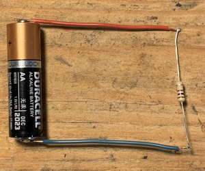
Figure 2.9 Circuit #1, consisting of an AA battery, resistor, and conducting wires

We assume, at this point, that the red and green connecting wires seen in this photo are perfectly conducting. (We will define this term and discuss the small resistance of these wires in a subsequent section.) The battery causes a current to flow in the circuit, with charges exiting the battery’s + terminal, traveling through the top wire, down through the resistor, and returning through the lower conductor to the battery’s – terminal. The battery in this circuit serves as the force that causes the charges to flow clockwise around the circuit loop. The battery is a source of energy, while the resistor is a consumer of energy or an energy sink. Positive electrical charges flowing clockwise in the circuit transfer energy from the battery into the resistor. Because of the perfectly conducting wires, the $1.5 V$ potential difference (that is, the voltage) across the battery terminals is applied directly across the resistor, so that the upper terminal of the resistor is at an electric potential $1.5 \frac{J}{C}$ higher than the lower terminal of the resistor. We can consider energy transfer by considering what happens around the circuit loop starting with the $-$ terminal of the battery: charges enter the $-$ terminal and exit the $+$ terminal of the battery, gaining $1.5$ Joules of energy per coulomb of charge; charges then move through the upper conductor with no change of energy; they then enter the upper terminal of the resistor, which is at a potential $1.5 V$ higher than the resistor’s lower terminal. Passing through the resistor, every coulomb of charge loses $1.5 J$ of energy owing to the $1.5\frac{J}{C}$ (or $1.5 V$ ) voltage drop across the resistor. Inside the resistor, the energy from the charges is converted to heat. This happens when atoms within the resistor are caused to accelerate and collide with one-another. Usually, we will not concern ourselves with what is happening inside a device; instead, we will concern ourselves with how the device behaves when it is connected to other elements in a circuit. Leaving the lower terminal of the resistor, the charges move through the lower conductor then re-enter the $-$ battery terminal, thereby completing the loop.

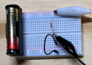
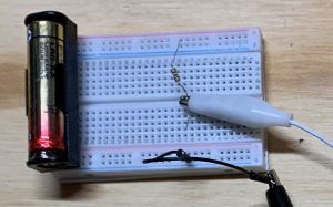
Voltage and current measurement using a multimeter. Later in this book, we will work with circuits that have actuators in them including diodes that emit light and motors that spin, which give us an obvious indication that the circuit is doing something. If we attached a temperature probe to the resistor in the circuit described above, we would find that this circuit is doing something: it is heating the resistor. We can also measure the goings-on of this circuit by using a multimeter to measure voltage and current. Circuit#1 is shown below, after having been re-assembled onto a solderless breadboard. A pair of alligator clip-leads is attached across the ends of the resistor and attached to the red (+) and black (-) probes of the digital multimeter, which is set up to measure DC voltage. The voltage drop across the resistor, which also corresponds to the battery voltage, is 1.59 V. This is a typical value for a new AA battery.

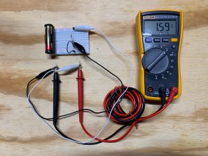
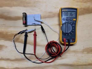
Figure 2.10a Alligator clips attached to the two ends of the resistor for measuring voltage “across” the resistor

Figure 2.10b Circuit #1 assembled onto a solderless breadboard and a digital multimeter set up to measure the voltage across the resistor

The same digital multimeter can be used to measure the current flowing in the circuit loop by setting the meter to read DC current, moving the red probe of the meter into the current-measuring socket, breaking open the circuit, and letting the current flow through the meter as shown. The current is 0.016 A or 16 mA. In the next chapter we will discuss several circuit laws that explain why a 1.5 V battery and 100 Ω resistor result in this value of current.

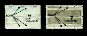
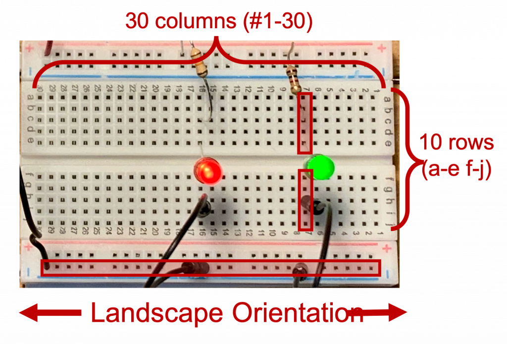
Figure 2.11a Alligator clips attached to one resistor lead and to the ground rail for measuring the current “through” the circuit loop

Figure 2.11b Circuit #1 on the breadboard with the multimeter set up to measure the current flowing through the resistor

Solderless breadboards. The implementation, or the construction, of the circuit on the solderless breadboard can be understood by examining figure 2.12 showing the top surface and underside of a breadboard. We orient breadboards with the long dimension horizontally and the shorter dimension vertically. In this “landscape” orientation, shown in figure 2.13, (as opposed to “portrait” orientation, shown in figure 2.14), we see that the breadboard is comprised of rows and columns of interconnected connection points that allow wires and components to plug in, The top and bottom two rows serve as “power rails” and are, by convention, used to connect the voltage supply to the components. In the previous circuit, the + terminal of the battery is connected to the red voltage rail, while the – terminal is connected to the blue voltage power supply rail. The breadboard also has numerous vertical columns, each containing 5 connected wire insertion points. This will make more sense as we assemble progressively more complicated circuits on breadboards beginning with the next chapter.

Figure 2.12 Solderless breadboards are oriented with the long dimension horizontal. Conducting rows and columns are individually connected underneath the breadboard as seen on the right.

Figure 2.13 Breadboard in landscape orientation has 300 grid points: 10 rows x 30 columns

Figure 2.14 Some references use portrait orientation for breadboards with 30 rows and 10 columns. This text does not used this orientation.

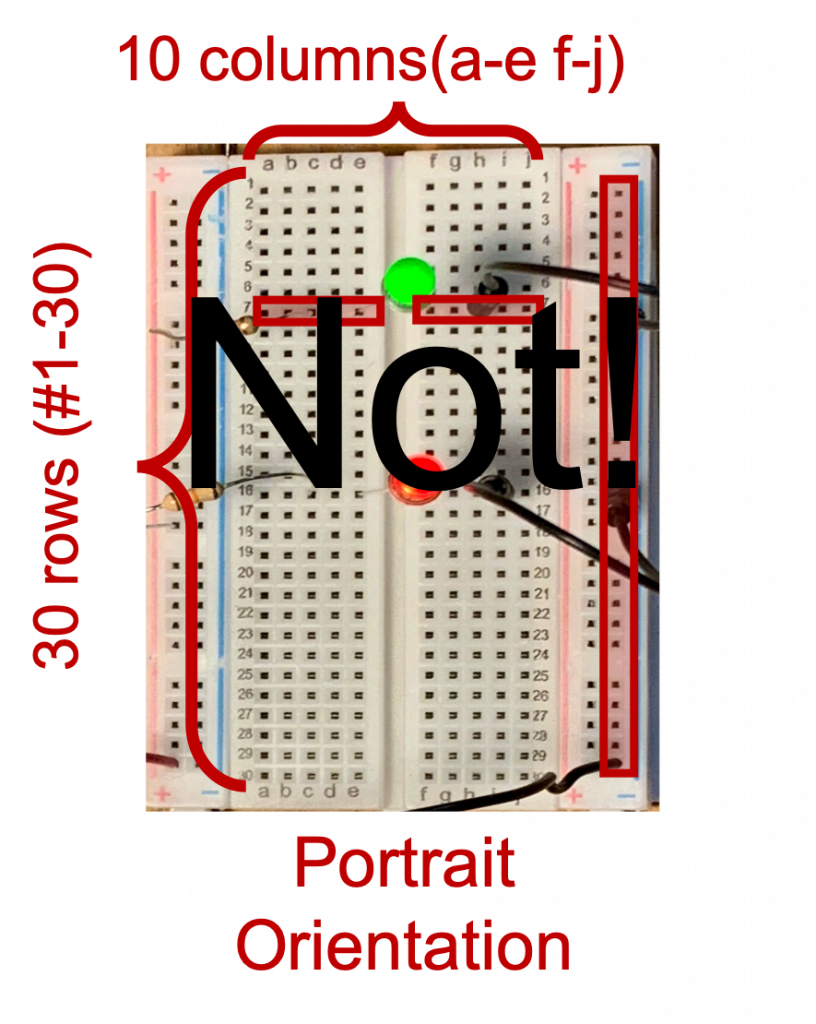
The following video was created by Lizzy McEleney, a student in ECE361 during Fall 2017, to describe how to use solderless breadboards and digital multimeters. Note that this video uses a portrait orientation, in which the designations for rows and columns are reversed.

Lizzy McEleney’s video on breadboards and DMMs

Warning: A common mistake made by students in their initial experiments with a multimeter is to set up the meter to measure current, while placing the meter probes across a device, rather than breaking the circuit and letting current flow through the meter. This results in a large current flowing through the meter and in many cases either blows the fuse in the meter or, worse, damages the meter. We will discuss this in more detail in the Lab One assignment section. For now, view Lizzy’s video and be warned.

Electric and fluid circuit analogy. It can be helpful to compare circuit#1 to a hydraulic analog of a pump driving fluid around a closed loop of pipes.

Figure 2.15 Hydraulic system with pump driving fluid around a closed loop of pipes

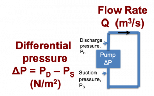
A mechanical pump forces fluid to move around the closed hydraulic loop at a certain flow rate. The low-pressure, or suction end of the pump, pulls in fluid, while the high-pressure, or discharge end, pushes fluid out. The resulting fluid circulates around the circuit in a clockwise direction. The pump is characterized by its differential pressure, $\Delta P$ which is the discharge pressure minus the suction pressure,

(1) $\begin{equation*} \Delta P= P_{D} - P_{S} \end{equation*}$

and has units of Pascal or $\frac{N}{m ^{2}}$ . By dimensional analysis,

(2) $\begin{equation*} \frac{N}{m^{2}}=\frac{N \cdot m}{m^{3}}=\frac{J}{m^{3}} \end{equation*}$

we see that the differential pressure can be interpreted as the increase in energy, per $m^{3}$ , or per unit volume, as fluid travels through the pump. The increased energy forces the fluid to flow through the pipes, where energy is given up via pipe resistance and converted into heat. The flow-rate of the fluid, $Q$ in $\frac{m^3}{s}$ (in the imperial measurement system, $\frac{gallons}{minute}$ would be used; we use the MKS system in this text, unless otherwise noted) is determined by the diameter of the pipes, with larger diameter pipes having higher flow rates. The product of the differential pump pressure and the flow rate is the power of the circuit,

(3) $\begin{equation*} P = \Delta P \cdot Q \end{equation*}$

having units of watts (W):

(4) $\begin{equation*} \frac{J}{m^{3}} \cdot \frac{m^{3}}{s} = \frac{J}{s} = W\end{equation*}$

This corresponds to the rate at which the pump delivers energy to the fluid. A small recirculating pump, for example, with a capacity of $\frac{1}{3} hp$ has an MKS capacity of $745.7 \frac{W}{hp} \cdot \frac{1}{3} hp = 248.6 W$ . Such a pump transfers `~ $250 J$ of energy each second into the fluid.

Comparison between the two circuits: we now return to our simple battery and resistor electric circuit, represented below by a schematic circuit drawing. In this schematic, the battery and resistor are represented by symbols and the conducting wires are represented simply as lines. We shall say more about schematics as we proceed through the text.

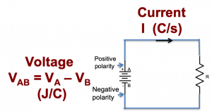
Figure 2.16 Electrical system with battery driving current around a closed loop if wires and resistance

The electric potential difference, or voltage, between the positive battery terminal A and the negative terminal B, is given by:

(5) $\begin{equation*} V_{AB}= V_{A} - V_{B} \end{equation*}$

and has units of

(6) $\begin{equation*} \frac{J}{C} \end{equation*}$

we see that the potential difference can be interpreted as the increase in energy, per $C$ , as charges flow through the battery. The increased energy forces the charges to flow through the circuit, where energy is given up via resistance and converted into heat in the resistor. Comparison of equations (2) and (6) reveals that each represents energy transfer to the flow in the circuit: joules per unit fluid volume of in the hydraulic case and joules per unit electrical charge in the electric case. The battery and the pump serve as the forcing mechanisms to drive current flow, and fluid flow around their respective circuits. The electrical current $I$ in $\frac{C}{s}$ is analogous to the fluid flow rate Q in $\frac{m^{3}}{s}$ .

The product of battery voltage and electrical current is analogous to the product of pressure differential and flow rate; in both cases, this product is the power of the system, or the rate at which energy is transferred. The product of the voltage and the current is,

(7) $\begin{equation*} P = V_{AB} \cdot I \end{equation*}$

having units of watts:

(8) $\begin{equation*} \frac{J}{C} \cdot \frac{C}{s} = \frac{J}{s} = W\end{equation*}$

This corresponds to the rate at which the battery delivers energy to the system. Referring back to figure 2.9 and circuit#1, the $1.5V$ battery voltage and $0.016 A$ circuit current represent a power of $0.024W$ , meaning $0.024 J$ of energy is supplied by the battery every second and consumed by the resistor as heat.

Energy Transfer. Energy is transferred when charge flows through a circuit element having a voltage across its terminals. Consider the circuit shown in figure 2.17. A positive charge entering the $-$ terminal of the $1.5 V$ battery exits the $+$ terminal with an increase in energy of $1.5 \frac{J}{C}$ . Conversely a charge entering the $+$ terminal of the resistor and exiting the $-$ terminal experiences an energy decrease of $1.5 \frac{J}{C}$ . A current of $0.1 A$ or $100 mA$ flows clockwise through this particular circuit (we will calculate this using Ohm’s law later in this chapter). The power associated with the battery and the resistor is $1.5 V \cdot 0.1 A = 0.15 W$ . We can say that the resistor absorbs $0.15W$ and the battery absorbs $-0.15W$ , the negative sign here representing the fact that the battery is actually supplying power rather than absorbing it.

Figure 2.17 Battery is the source of energy while the resistor is the consumer of energy

This process of energy transfer would continue until the battery is depleted of all of its energy. An alkaline AA battery has ~ $10kJ$ of energy when new; if energy is consumed at a rate of $0.15\frac{J}{s}$ the battery would last $\frac{10000}{0.15}=66,667 s$ or $18.5 hours$ and then it would be time to discard the battery. Primary batteries such as the ones shown on this page are disposed of when their energy is depleted. Energy-depleted secondary or “rechargeable” batteries can have their energy replenished by the process commonly known as “battery charging”. It is important to note that the term “recharging” a battery means adding energy back into the battery; “recharging” has nothing whatsoever to do with the addition of charge to the battery.

A fresh alkaline AA battery has ~ $10kJ$ of energy. Primary batteries are not rechargeable. Secondary batteries can be recharged. The term “recharging” a battery means adding energy back into the battery; “recharging” has nothing whatsoever to do with the addition of charge to the battery.

Want to learn more about batteries? Check out: https://batteryuniversity.com/articles

also go back to chapter 1 and check out the data sheets for the batteries contained in your lab kit.

Examples

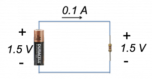
Example: How much power is absorbed by each element in the circuit shown?

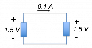
Solution: Each element has a voltage of $1.5 V$ and a current of $0.1 A$ , so the power associated with each element is $1.5 \cdot 0.1 = 0.15 W$ . Since the current flows clockwise through the circuit, charges are gaining energy from the circuit element on the left and giving up energy to the circuit element on the right. Therefore, the element on the left is absorbing $-0.15W$ while the element on the right is absorbing $0.15 W$ .

Pause for a minute and think about this. This is the same circuit as the battery & resistor circuit shown in figure 2.17; based on the discussion above, we know that the battery is supplying $0.15 W$ of power. We can equivalently say that the battery is absorbing $-0.15W$ , and we know from our discussion above that the resistor is absorbing $0.15W$ . Suppose we come upon this problem without prior knowledge that the circuit element on the left is a battery, an energy source, and that the circuit element on the right is the energy sink? The solution is to follow the current and the voltage drops and rises: the current is flowing clockwise in the circuit, as indicated by the direction of $0.1A$ arrow. The circuit element on the right has a voltage drop of $1.5V$ : the charges enter the $+$ terminal of the circuit element, and they exit the $-$ terminal after having given up $1.5 J$ of energy per coulomb of charge. The element on the right is therefore a consumer, a sink, or an absorber of energy. Continue to follow the charges as they experience a voltage rise in the circuit element on the left: they enter the $-$ terminal of the element then exit the $+$ terminal after having gained $1.5V$ or $1.5$ joules of energy per coulomb of charge. The circuit element on the left is, therefore, a source of energy. This is a central idea behind this whole book and you should stay with it until it makes sense to you.

Still not getting it? A gravitational analogy might be helpful. Think of the upper wire in this circuit as a frictionless surface elevated above the ground, and think of the lower wire as another frictionless surface at ground level. Imagine a smooth object (a book, a hockey puck, a baseball, or whatever) moving along the “circuit” from left to right in the upper level, down to the lower level, then moving from right to left, back to the upper level, and continuing. One of the circuit elements must be the source of energy that lifts the object from ground level to the upper level, increasing its potential energy as it lifts. This element could be you; you are the energy source. The other element transfers the elevated potential energy into kinetic energy as the object moves from the higher elevation to the ground. This element could simply be the “bang” heard then the object is dropped, accelerates, and slams into the ground. This is the energy sink or absorber.

Example: A circuit element has voltage of $10V$ between its terminals as shown. A positive charge of $5 C$ moves through the circuit from terminal $a$ to terminal $b$ . How much energy is transferred? Is the energy supplied by the circuit element or absorbed by it?

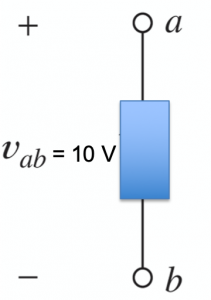
Solution: The charges are moving from higher to lower potential, so they lose $10 \frac{J}{C}$ as they move from terminal $a$ to terminal $b$ . Since $5 C$ of charge is transferred, $5 C \cdot 10 \frac{J}{C} = 50 J$ of energy is lost by the charges. This energy is absorbed by the circuit element.

License

Icon for the Creative Commons Attribution 4.0 International License

Applied Electrical Engineering Fundamentals by David J. McLaughlin is licensed under a Creative Commons Attribution 4.0 International License, except where otherwise noted.

License

Share This Book