2.1 Basic Physics Review

David J. McLaughlin

2.1 Basic Physics Review

This section reviews the concepts of electric charge and electric potential (also known as voltage). Electric charge is a measure of quantity of electricity and can have positive or negative values. Recall that matter is made up of atoms which, in turn, are made of negatively charged electrons, positively charged protons, and neutrally charged neutrons. Recall from your physics class that electrical charges exert forces on each other analogous to the way masses attract each other and give us gravity. More than one engineering student has reported that mass and gravity are more familiar and less abstract concepts than charge and electric potential. This may be pervasive: we may not understand relativistic effects and curvature in the space-time continuum, but all engineering students are comfortable applying Newton’s law of gravitation to compute the attractive force between two masses in the Universe. Many engineers use these concepts to analyze material strain and build bridges and skyscrapers. Even though light (electromagnetic energy) is visible all around us, electromagnetics just seems to be harder to digest. So we start this discussion with mass and gravity and then move to the analogous context, where the formulas are nearly the same, and we examine charge and electric potential. Simple expressions for gravitational attraction as well as gravitational and electric potential are given below as a way to help illustrate concepts. We are not interested in computing these quantities in any detail in this course, however.

Gravitational attraction. Recall that objects having mass exert attractive forces on one-another via the uniform law of gravitational attraction. Assume we have a small “test mass”, $m_{t}$ , separated from another small mass, $m$ by distance $r$ . As illustrated in Fig. 2.1, mass $m$ exerts an attractive force on mass $m_{t}$ given by

(1) $\begin{equation*} F=\frac{Kmm_{t}}{r^{2}} \end{equation*}$

in units of Newtons (N) where the gravitational constant $K=6.674\cdot10^{-11} m^{3} \cdot kg^{-1} \cdot s^{-2}$ . (Likewise, mass $m_{t}$ exerts an attractive force on mass $m$ . However, let us concern ourselves only with the force on our test mass, $m_{t}$ .)

Figure 2.1 Mass m exterts an attractive force on the “test mass” $m_{t}$ .

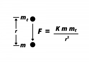If we let $m=5.972 \cdot 10^{24} kg$ , the mass of the Earth, and we let $r=6.378 \cdot 10^{6} m$ , the radius of the Earth, and we insert these values into equation (1) then we have

(2) $\begin{equation*} F=m_{t}g \end{equation*}$

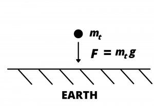
which is the familiar equation for the attractive force due to gravity, where $g=9.8 N \cdot kg^{-1}$ . This is depicted in Fig. 2.1 and is really an approximation, valid for objects close to the Earth’s surface. In this figure, the Earth’s surface is shown as being flat rather than spherical; this is due to the fact that the Earth’s radius is so large that any sketch of its surface up close appears flat.

Figure 2.2 Gravitational attraction by the Earth’s mass on test mass $m_{t}$ .

Gravitational potential energy. Now consider test mass, $m_{t}$ , at two different heights above the surface of the Earth, $h_{A}$ and $h_{B}$ as shown. At these two heights, the mass has potential energy

(3) $\begin{equation*} E_{A}=m_{t}gh_{A} \end{equation*}$

in joules (J) and

(4) $\begin{equation*} E_{B}=m_{t}gh_{B} \end{equation*}$

as illustrated in Fig. 2.2

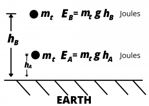Figure 2.2 Potential energy of our test mass $m_{t}$ at two different heights above the earth (or ground).

The work needed to lift the mass from height h_A to height h_B is

(5) $\begin{equation*} E_{BA}=m_{t}g(h_{B}-h_{A}) \end{equation*}$

Thus $E_{BA}$ represents the amount of energy that would need to be transferred into the mass at height $h_{A}$ in order to bring it up to height $h_{B}$ . (Where does the energy come from? If the object is a text book being lifted from the floor to a table top, then the person doing the work to lift the book is providing the energy). This energy is said to be stored in the potential energy of the mass at height $h_{B}$ relative to height $h_{A}$ . The energy is stored in the sense that it can be released, and converted into kinetic or other energy forms by allowing the mass to move from h_B down to height $h_{A}$ . (Back to the book-on-the-table: assume h_B represents the height of the table and h_A represents the height of the floor. If we push the book off the table, it will fall to the floor, accelerating as it falls and as potential energy is converted into increasing kinetic energy. When the book hits the floor, the kinetic energy is absorbed in the impact, with some of the energy being converted into heat and some being converted into acoustic energy as the book makes a “bang” noise. Staying with the book-on-table example just a bit more: it is important to realize that it is the difference in heights, $h_{B}-h_{A}$ that matters here rather than the actual heights themselves. If the table were placed outside, on the actual ground, then $h_{A}$ would actually represent ground-level while $h_{B}$ would be the height of the table above ground. If that same table were to be placed atop the tallest building, $h_{A}$ would be the height of the building above the ground, and $h_{B}$ would be represent the additional height above the table sitting atop that building. The energy needed to lift the book to the table top, and the energy released when the book is pushed off the table top, is the same in both cases.)

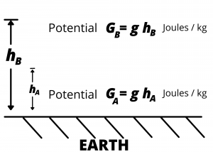
Gravitational potential. Another way of characterizing the gravitational field is via the gravitational potential, G, having units of energy per unit mass, $\frac{N\cdot m}{kg}$ or $\frac{J}{kg}$ . The gravitational potential at heights $h_{B}$ and $h_{A}$ is, simply, $gh_{B}$ and $gh{A}$ , respectively. Moreover, the difference in gravitational potential, the gravitational potential difference, when multiplied by $m_{t}$ , gives the work needed to lift the mass from height $h_{A}$ to height $h_{B}$ . We have introduced this seemingly abstract concept because its electrical analog, the electric potential difference, also known as voltage, is used constantly when dealing with electrical circuits. If we introduce a mass above the earth’s surface at a given height, it is attracted downward, toward lower gravitational potential. If the mass were released at height $h_{B}$ , it would fall toward lower height $h_{A}$ and give up potential energy as it fell. Conversely, if the mass is caused to increase in height by some external force, such as our hand lifting it, then the mass would absorb energy from our lifting hand as it moves from lower to higher gravitational potential.

Figure 2.4 Gravitational potential at different heights

A mass gains potential energy as it moves from lower to higher gravitational potential. Conversely, a mass gives up potential energy as it moves from higher to lower gravitational potential.

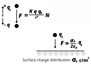
Electrostatic attraction. Consider two small charged particles: a test particle having positive charge + $q_{t}$ coulombs (C) and another particle having negative charge $-q$ C separated by a distance $r$ . We consider a positive and a negative charge so that there is an attractive force between them, analogous to gravitational attraction between two masses. Coulombs law specifies that the test charge $q_{t}$ experiences a force of attraction $F$ , due to $-q$ given by the relationship:

(6) $\begin{equation*} F=\frac{Kqq_{t}}{r^{2}} \end{equation*}$

where in this case, $K$ is Coulomb’s constant $K=9\cdot10^{9} N\cdot m^{2} \cdot C^{-2}$ .

Note the similarity between the attractive force equations (1) and (6). If we were to replace particle $-q$ with a large two-dimensional surface characterized by a surface charge distribution $-\sigma_{s} \frac{C}{m^{2}}$ then the attractive force on test charge $q_{t}$ would be

(7) $\begin{equation*} F=\frac{\sigma_{s}}{2\epsilon_{0}} \end{equation*}$

The constant $\epsilon_{0}$ is referred to as the permittivity of free space. Compare figure 2.5 with figures 2.1 and 2.2 and also note the similarity between this equation and equation (2), which again helps to show the analogy between the electrical and mass-attraction cases. While we might lack an intuitive sense for a “two-dimensional surface charge distribution” we can appreciate this case by analogy to the gravitational case described above.

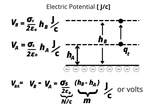
Figure 2.5 Electrostatic attraction by a charge -q (left) and a surface charge distribution (right). Each exerts an attractive force on a test charge

Analogous to the gravitational potential discussed above, we can also define electric potentials $V_{A}$ and $V_{B}$ , such that the difference in these potentials, $V_{A}-V_{B}$ , represents the energy needed per unit charge to move (“lift”) a charged particle from height $h_{A}$ to height $h_{B}$ above the charged surface. Note that this is analogous to lifting a mass against the force of gravity, only in this case, the particle is “lifted” against the attractive force of the surface charges. The surface charge distribution maintains an electric potential difference $V_{B}-V_{A}$ in the space between $h_{A}$ and $h_{B}$ , with the result that a test charge either gains or loses energy when moving between these two heights.

Figure 2.6 Electric potential at two distances (or heights) from a surface charge distribution

We know that electric charges can have both positive and negative sign. Now consider a region of space characterized by a positive surface charge distribution above a negative surface charge distribution.

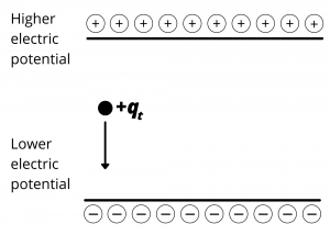
Figure 2.7 Electric potentials associated with two surface charge distributions

A positive charge placed in this region would be attracted downward by the attractive force of the negative charges on the lower surface and the repulsive force of the positive charges on the upper surface. Energy would need to be supplied to the charge to lift it upward toward the positive surface, indicating the positive surface is the region of higher electric potential. Conversely, if a charge were released, it would “fall” toward lower electric potential as it is attracted toward the negative charge distribution.

If this were a course in physics or electromagnetics we would likely be concerned with calculating the forces, fields, and potentials of various types of charge distribution. That is not our purpose here; this section is presented simply to familiarize ourselves with charges and electric potentials, so as to get a “running start” into the next section. The key take-away point from this chapter is this: charges gain electric potential energy when they go from lower to higher electric potential ( $\frac{J}{C}$ ) just as masses gain gravitational energy (PE) when they go from lower to higher gravitational potential ( $\frac{J}{kg}$ ). Conversely, charges give up energy when they move from higher to lower electric potential, just as masses give up energy when they move from higher to lower gravitational potential.

License

Icon for the Creative Commons Attribution 4.0 International License

Applied Electrical Engineering Fundamentals by David J. McLaughlin is licensed under a Creative Commons Attribution 4.0 International License, except where otherwise noted.

License

Share This Book