6.4 Negative Feedback Amplifier

David J. McLaughlin

6.4 Negative Feedback Amplifier

Op amp circuits can achieve controlled voltage gain while avoiding saturation by employing negative feedback. The basic idea is to provide a path between the op amp output node, which has voltage V_o, and the inverting terminal input node, which has voltage V_–. In the example circuit shown in figure 6.22, this is accomplished via the feedback resistor R_f.

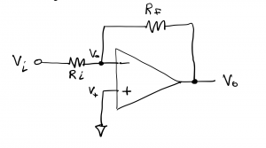
This feedback path serves to subtract part of the output voltage from the differential input voltage as a way to avoid saturation by the very high gain amplifier, A. The impact of feedback is to drive the differential input voltage (V₊-V_–) toward a very small value (ideally, zero). When multiplied by the very large (ideally, infinite) open-loop gain, $A$ , the output voltage $V_{0}$ remains finite and the op amp avoids saturation. Read the last three sentences again and think about what is written. Repeat.

How negative feedback works. We begin by considering the closed-loop feedback amplifier block diagram shown in figure 6.23. This circuit has the same function as the op amp circuit shown above, but it is implemented more simply with three functional blocks (when we say “functional” we mean that we will concern ourselves with what the block does, rather than what the block is or how the functionality is achieved; we don’t care what’s inside the block): a difference block that subtracts one signal from another, and two amplifier blocks, a forward amplifier having gain A and a reverse, or backward amplifier, having gain f. (Forward and backward just refer to the input-output flow direction of the amplifiers: left to right in the forward case and right to left in the backward case.) The amplifier blocks simplify multiply their respective inputs by A and f to produce output signals. Given these definitions, we can readily derive the input-output relationship, $V_{o}$ vs. $V_{i}$ for this circuit by inspecting the block diagram:

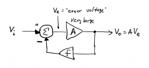
$V_{e}$ , defined as the “error voltage”, is the difference between the input signal $V_{i}$ and the output signal $V_{o}$ , having been amplified by backward gain f. This is called an error voltage in control theory because it often represents the difference between a desired value and an achieved value. As we shall see, this voltage is driven to zero by the feedback circuit.

The error voltage is given by

(1) $\begin{equation*} V_{e}=V_{i}-fV_{o} \end{equation*}$

$V_{o}$ is an amplified version of the error voltage,

(2) $\begin{equation*}V_{o}=AV_{e}\end{equation*}$

Substituting, eq. (1) into eq. (2) we have

(3) $\begin{equation*} V_{o}=A(V_{i}-fV_{o})=AV_{i}-AfV_{o} \end{equation*}$

from which we obtain, via algebraic manipulation:

(4) $\begin{equation*} V_{o}(1+Af)=AV_{i} \end{equation*}$

and then

(5) $\begin{equation*} V_{o}=\frac{AV_{i}}{(1+Af)} \end{equation*}$

We know that op amps have very large (ideally, infinite) values of A, so we want to examine the behavior of this input-output relationship for very large A. To do this, we divide numerator and denominator by A, achieving

(6) $\begin{equation*} V_{o}=\frac{V_{i}} {(\frac{1}{A}+f)} \end{equation*}$

The closed-loop gain is given by

(7) $\begin{equation*} G=\frac{V_{o}}{V_{i}}=\frac{1}{\frac{1}{A}+f} \end{equation*}$

when we let A become very large, $1/A$ becomes negligible and we have

(8) $\begin{equation*} G\approx\frac{V_{o}}{V_{i}}=\frac{1}{f} \end{equation*}$

For the ideal op amp with A=∞, eq. (8) is an equality rather than an approximation since $\frac{1}{A}=0$ .

Note that the closed-loop gain of the circuit, $1/f$ , is independent of gain $A$ . All that was required was that $A$ be very large compared with $1/f$ . $A$ , which we refer to as the open-loop gain, serves an important role in the circuit, but its precise value is not important. The closed-loop gain of the circuit is determined entirely by $f$ . (In the example below, we will examine the impact of different values of $A$ on a circuit.)

Recall that the relationship between the error voltage and the output voltage is: $V_{o}=AV_{e}$ from which we see that $V_{e}=V_{o}/A$ . Since $A$ is very large (ideally, infinite), $V_{e}$ is very small (ideally, zero). From this information, we can make the following inference about the behavior of a feedback circuit such as this: the very large gain of the forward amplifier, $A$ combined with feedback amplifier gain $f$ and a difference-forming circuit results in a gain of $1/f$ independent of $A$ . An important point is that the forward amplifier $A$ is prevented from saturating due to the feedback mechanism which drives the error voltage toward zero.

Example: in the previous problem, assume $A=10^{6}, f=0.1$ , and $V_{i}=1$ . Assume the circuit is powered by a 12 volt unipolar source. Does the amplifier saturate? Why or why not? Determine $V_{e}$ and $V_{o}$ as well as the closed loop gain of the amplifier, $G$ . Repeat for $A=\infty$ .

Solution: For $A=10^{6}$ , the closed loop gain, $G=\frac{ 1}{\frac{1}{A}+f}= 9.9999$ . For an input $V_{i}=1$ volt, the output voltage $V_{o} = GV_{i} = 9.9999*1 = 9.9999V$ ≈10 V. The error voltage in this case is $V_{e}=\frac{V_{o}}{A} = \frac{9.9999}{10^{6}}= 10^{-5}V$ . The forward amplifier $A$ does not saturate, since the product $V_{e}A=10^{-5}\cdot10^{6}=10$ indicating that the output voltage is kept below the $12$ volt power supply rail and the amplifier $A$ is operated in its linear region.

For $A=\infty$ , the closed loop gain, $G=\frac{1}{f} = 10$ . The output voltage $V_{o} = GV_{i} = 10\cdot1 = 10 V$ . The error voltage is $V_{e}=\frac{V_{o}}{A} = 0$ . The forward amplifier does not saturate because the output voltage is kept below the power supply rail.

Now let us take the previous discussion and apply to to the op amp circuit that has a feedback resistor connecting $V_{o}$ to $V_{-}$ .

We are interested in deriving the input – output relationship for this circuit, $V_{o}$ vs $V_{i}$ , from which, we will determine the closed-loop gain, $G=\frac{V_{o}}{V_{i}}$ . We use the equivalent circuit shown to analyze this circuit using circuit analysis rules. The equivalent circuit replaces the op amp’s “triangle” symbol with a dependent source at the output, and we assume infinite input resistance and zero output resistance. This model is only valid when the op amp is operated within its linear region of operation (ie, it is not saturated); so we will need to verify that voltage levels are kept within this region.

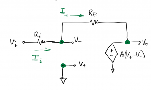
The input voltage to this circuit, V_i, is known and the other node voltages, V_–, V₊, and V_o, need to be determined. We can use the technique of node voltage analysis to determine these voltages. We can see that

(9) $\begin{equation*} V_{+}=0 \end{equation*}$

since the non-inverting terminal is connected directly to a ground node. Since V_o is connected directly to the + terminal of the dependent voltage source, and since V₊=0, we have

(10) $\begin{equation*} V_{o}=A(V_{+}-V_{-})= -AV_{-} \end{equation*}$

Now we apply KCL at node V_– as we practiced when studying node voltage analysis:

(11) $\begin{equation*} I_{i}=I_{f} \end{equation*}$

(12) $\begin{equation*} \frac{V_{i}-V_{-}}{R_{i}}=\frac{V_{-}-V_{o}}{R_{f}} \end{equation*}$

substituting $V_{-} = \frac{-V_{o}}{A}$ we have

(13) $\begin{equation*} \frac{V_{i}+\frac{V_{o}}{A}}{R_{i}} = \frac{\frac{-V_{o}}{A}-V_{o}}{R_{f}} \end{equation*}$

which gives, after some algebra,

(14) $\begin{equation*} V_{o}=\frac{V_{i}R_{f}}{\frac{-R_{i}}{A}-R_{i}-\frac{R_{f}}{A}} \end{equation*}$

The closed-loop gain of the overall resulting circuit,

(15) $\begin{equation*} G=\frac{V_{o}}{V_{i}}=\frac{R_{f}}{\frac{-R_{i}}{A}-R_{i}-\frac{R_{f}}{A}} \end{equation*}$

since $A$ is large, we can ignore terms involving $\frac{1}{A}$ to obtain an approximate expression for closed loop gain,

(16) $\begin{equation*} G\approx\frac{-R_{f}}{R_{i}} \end{equation*}$

Note this this expression for $G$ is exact when we have an ideal op amp with $A=\infty$ .

The differential input signal is related to the output voltage by

(17) $\begin{equation*} V_{o}=A(V_{+}-V_{-}) \end{equation*}$

Rearranging, we see that

(18) $\begin{equation*} V_{+}-V_{-}=\frac{V_{o}}{A} \end{equation*}$

and with $A$ very large (ideally, zero), the differential input voltage

(19) $\begin{equation*} V_{+}-V_{-}\approx 0 \end{equation*}$

and, when $A=\infty$ , the approximation becomes an equality. This is due to the presence of the feedback resistor connecting $V_{o}$ to $V_{-}$ . Although we have developed this result and observation in the case of the particular negative feedback Op Amp circuit shown in figure 6.24, the results here do apply for all negative feedback op amp circuits. This result leads to an important observation that negative feedback in an Op Amp circuit causes the differential input voltage to become negligible. This observation, referred to as the Summing Point Constraint, or Virtual Short Circuit, leads to a quick and simple way to analyze negative feedback op amp circuits, namely:

- confirm the presence of a negative feedback path between $V_{o}$ and $V_{-}$
- apply the summing point constraint: $V_{+} = V_{-}$
- recall that the input currents flowing into the + and – terminals of the op amp are negligible.

We can apply this technique to the analysis of the inverter circuit that we examined above:

Since there is negative feedback, via $R_{f}$ , the summing point constraint tells us that V_–=V₊. Since the non-inverting terminal of the op amp is connected to ground, we have

(20) $\begin{equation*} V_{-}=V_{+}=0 \end{equation*}$

Applying KCL at the op amp inverting input terminal, we have

(21) $\begin{equation*} I_{i}=I_{f} \end{equation*}$

where $I_{i}$ is the current through $R_{i}$ and $I_{f}$ is the current through $R_{f}$ . By Ohm’s law, we can write

(22) $\begin{equation*} \frac{V_{i}-0}{R_{i}} =\frac{0-V_{o}}{R_{f}} \end{equation*}$

which simplifies to

(23) $\begin{equation*} \frac{V_{i}}{R_{i}} =-\frac{V_{o}}{R_{f}} \end{equation*}$

and gives us the gain of the amplifier circuit,

(24) $\begin{equation*} G=\frac{V_{o}}{V_{i}} =\frac{-R_{f}}{R_{i}} \end{equation*}$

Examples

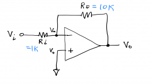
Example: Determine the closed-loop gain of the op amp circuit shown assuming $A=\infty$ . Determine voltages $V_{-}, V_{+}, V_{o}$ , as well as currents $I_{i}$ and $I_{f}$ , assuming an input voltage $V_{i}= 2$ volts and assuming the op amp is powered by a $24V$ unipolar supply voltage.