3.4 Node Voltage Analysis

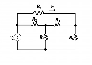
David J. McLaughlin; William C. Howe (2025 updates)

3.4 Node Voltage Analysis

Node voltage analysis is a systematic method for analyzing circuits based on determining the voltages at all circuit nodes relative to a reference, or ground node, in the circuit. To motivate this analysis method, consider the circuit shown in Figure 3.26. The circuit has 6 elements, including a known voltage source, $v_{0}$ , and five resistors having values $R_{1} - R_{5}$ . (Pretend we had actual numbers in place of the variables.) Consider the effort involved in determining all the voltages (five unknowns) and all the currents (six unknowns) in this circuit. Or, consider the effort involved in simply obtaining the current $i_{1}$ through resistor $R_{1}$ . There are no series or parallel-connected resistors in this circuit, so circuit simplification based on equivalent resistance does not help to simplify the work. We could solve this circuit by repeated application of KCL, KVL, and Ohm’s Law to solve for all the circuit unknowns. The circuit has 11 unknowns, so we would need to develop a system of 11 simultaneous linear equations by applying KVL, KCL, and Ohm’s law to the various loops, nodes, and resistors in the circuit. Solving this system of equations would, in principle, complete the circuit analysis problem. We develop these equations below to illustrate, by way of this example circuit, the effort involved in such a “brute force” application of circuit analysis laws. Then, we introduce node voltage analysis, which often leads to results with significantly less effort.

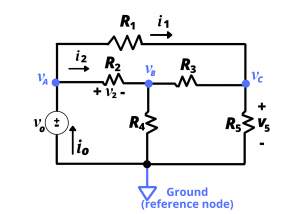
This circuit is re-drawn in figure 2.27 with annotations for: the voltage across and current through each circuit element, which are the sought-after variables; the four circuit nodes labeled A, B, C, D; several loops, namely, ABDA, BCDB, ACBDA, and DACD (these are not all of the possible loops). Writing Ohm’s law for the five resistors, applying KCL at the four nodes, and applying KVL around several circuit loops gives us a set of simultaneous equations.

This set of equations includes five Ohm’s law equations:

(1) $\begin{equation*} v_{1} = i_{1}R_{1} \end{equation*}$

(2) $\begin{equation*} v_{2} =i_{2}R_{2} \end{equation*}$

(3) $\begin{equation*} v_{3} =i_{3}R_{3} \end{equation*}$

(4) $\begin{equation*} v_{4} =i_{4}R_{4} \end{equation*}$

(5) $\begin{equation*} v_{5} =i_{5}R_{5} \end{equation*}$

in addition to four KCL equations, including KCL at node A,

(6) $\begin{equation*} i_{0} =i_{1}+i_{2} \end{equation*}$

KCL at node B,

(7) $\begin{equation*} i_{2} =i_{3}+i_{4} \end{equation*}$

KCL at node C,

(8) $\begin{equation*} i_{1}+i_{3} = i_{5} \end{equation*}$

and KCL at node D,

(9) $\begin{equation*} i_{4}+i_{5}= i_{0} \end{equation*}$

and five KVL equations, including KVL around loop ABDA,

(10) $\begin{equation*} -v_{0}+v_{2}+v_{4}=0 \end{equation*}$

KVL around loop BCDB,

(11) $\begin{equation*} -v_{0}+v_{2}+v_{4}=0 \end{equation*}$

KVL around loop ACBA,

(12) $\begin{equation*} v_{1}-v_{3}-v_{2}=0 \end{equation*}$

KCL around loop ACDA,

(13) $\begin{equation*} -v_{0}+v_{1}+v_{5}=0 \end{equation*}$

and (finally) KCL around loop ACBD,

(14) $\begin{equation*} -v_{0}-v_{3}+v_{4}=0 \end{equation*}$

Equations (1) – (14) represent a set of 14 simultaneous linear equations for this system. The system has only 11 unknowns, and we could have, in fact, written additional equations by including additional circuit loops (such as ABCDA). Algebraic manipulation of eq (1) – (14) (which we will not do here!) however would reveal they these equations are not all linearly independent. Among the four KCL equations, only three are independent, and the fourth can be derived from a linear combination of any three. The number of independent KCL equations is actually equal to the number of nodes in the circuit minus one. This circuit has four nodes, therefore, there are three independent KCL equations. Among the five KVL equations, only three are independent. (We could have listed a total of 7 KVL equations using loops ABDA, BCDB, ACBA, ACDA, ACBDA, ABCDA, and DBACD). The number of independent KVL equations is actual equal to the number of open areas in the circuit.

This circuit has three open areas, therefore, there are three independent KVL equations governing this circuit. Grouping together the five independent Ohm’s law equations, plus the three independent KCL equations, and three independent KVL equations, we would have 11 independent equations. Plugging in actual numbers for $v_{0}$ , $R_{1}$ , $R_{2}$ , $R_{3}$ , $R_{4}$ and $R_{5}$ and then solving this system of 11 equations would result in the 11 unknowns in the circuit. (Such fun!)

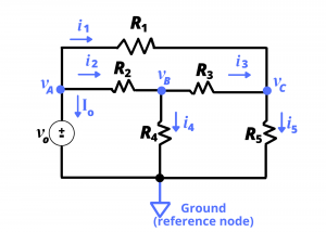
Node voltage analysis provides a simpler, more compact way to solve a circuit. Consider the same circuit again, but assume we already knew node voltages $v_{A}$ , $v_{B}$ , and $v_{C}$ relative to the reference (or ground) node. Assume we want to obtain $i_{1}$ , $i_{2}$ , $i_{0}$ , $v_{2}$ and $v_{5}$ . Given knowledge of node voltages $v_{A}$ , $v_{B}$ and $v_{C}$ relative to the ground node, consider the re-drawn circuit below:

We can readily write down the sought-after values in terms of the known node voltages:

(15) $\begin{equation*} i_{1} = \frac{(v_{A}-v_{C})}{R_{1}} \end{equation*}$

(16) $\begin{equation*} i_{2} = \frac{(v_{A}-v_{B})}{R_{2}} \end{equation*}$

(17) $\begin{equation*} i_{0} = i_{1}+i_{2} \end{equation*}$

(18) $\begin{equation*} v_{2} = v_{A}-v_{B} \end{equation*}$

(19) $\begin{equation*} v_{5} = v_{C} \end{equation*}$

It should be clear that knowing the node voltages permits the other circuit variables to be readily determined.

Determining the node voltages. Our circuit is reproduced in figure 3.30. We will use this figure to determine the node voltages.

Node voltage $V_{A}$ can be readily obtained by noting that this node is tied directly to the + terminal of voltage source $v_{0}$ , thus:

(20) $\begin{equation*} v_{A} = v_{0} \end{equation*}$

To solve for the remaining unknown node voltages, we use KCL:

KCL performed at node $v_{B}$ gives:

(21) $\begin{equation*} i_{2} = i_{3}+i_{4} \end{equation*}$

which can be re-written as

(22) $\begin{equation*} \frac{v_{A}-v_{B}}{R_{2}} = \frac{v_{B}-v_{C}}{R_{3}} +\frac{v_{B}}{R_{5}} \end{equation*}$

and, finally KCL performed at node $v_{C}$ gives:

(23) $\begin{equation*} i_{1} + i_{3}=i_{5} \end{equation*}$

which can be re-written as

(24) $\begin{equation*} \frac{v_{A}-v_{B}}{R_{1}}+\frac{v_{B}-v_{C}}{R_{3}} =\frac{v_{C}}{R_{5}} \end{equation*}$

Equations (20), (22) and (24) form a set of simultaneous linear equations that, when solved, gives us the node voltages $v_{A}$ , $v_{B}$ , and $v_{C}$ . For this particular circuit, since node voltage $v_{A}$ is always equal to the source voltage $v_{0}$ , $v_{A}$ is not an unknown variable, and the system of equations is quickly reduced to a system having two equations and two unknowns.

Any of the node voltages can be chosen as the ground or reference node. The ability to immediately write down $v_{A}=v_{0}$ illustrates why we happened to chose the particular ground node indicated in figure 3.30 as our reference node. This choice of ground node reduced the problem to solving for two unknown nodes rather than solving for three unknown nodes. Had we chosen $v_{C}$ as our reference node, we would still be able to analyze the circuit, but we would have needed to solve for three, instead of two, unknowns via a system of three, instead of two, simultaneous equations.

Examples

Example: Solve for the node voltages $V_{A}$ , $V_{B}$ and $V_{C}$ in the circuit below and then determine currents $I_{1}$ and $I_{2}$ .

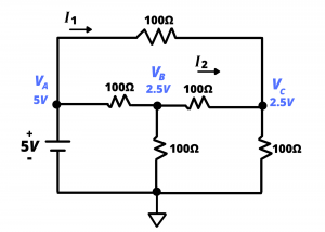
Solution: We can use eq. (20), (22) and (24) to solve this problem, inserting numerical values given in the circuit. Note that this system of three simultaneous equations is readily reduced to a system of two simultaneous equations since $V_{A}$ = 5 V. Inserting the numerical values for the circuit elements shown into equations (22) and (24) and solving these two equations simultaneously results in $V_{B}$ = 2.5 V and $V_{C}$ = 2.5 V. These voltages are annotated in red in the circuit drawing. With these voltages known, currents $I_{1}$ and $I_{2}$ are readily obtained:

$I_{1} = \frac{V_{A} - V_{C}}{100} = \frac{5-2.5}{100}$ = 0.025 V or 25 mV

and

$I_{2} = \frac{V_{B} - V_{C}}{100} = \frac{2.5-2.5}{100}$ = 0 V

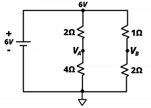
Example: In the circuit shown in figure 3.32 unknown node voltages $V_{A}$ and $V_{B}$ can be readily determined by recognizing that the two parallel branches loading the 6V battery are voltage dividers, with $V_{A}=6\frac{4}{4+2}=4V$ and $V_{B}=6\frac{2}{2+1}=4V$ .

Now consider figure 3.33 in which a resistance $x\Omega$ is connected between $V_{A}$ and $V_{B}$ . Use node voltage analysis to show that $V_{A}=V_{B}=4V$ regardless of the value of $x$ .

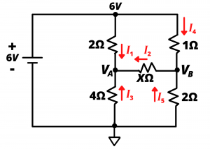
Solution: We begin by applying KCL at the node corresponding to $V_{A}$ which gives

(25) $\begin{equation*} I_{1}+I_{2}+I_{3}=0 \end{equation*}$

or

(26) $\begin{equation*} \frac{6-V_{A}}{2} +\frac{V_{B}-V_{A}}{x}}+\frac{0-V_{A}}{4}=0 \end{equation*}$

after algebraic manipulation to isolate $V_{B}$ on one side of the equation, we have

(27) $\begin{equation*} V_{B}=(1+\frac{3}{4}x)V_{A}-3x \end{equation*}$

Applying KCL at the node corresponding to $V_{B}$ gives

(28) $\begin{equation*} I_{4}-I_{2}+I_{5}=0 \end{equation*}$

or

(29) $\begin{equation*} \frac{6-V_{B}}{1} -\frac{V_{B}-V_{A}}{x}}+\frac{0-V_{B}}{2}=0 \end{equation*}$

and algebraic manipulation to isolate $V_{B}$ on one side of the equation results in

(30) $\begin{equation*} V_{A}=(1+\frac{3}{2}x)V_{B}-6x \end{equation*}$

Inserting eq (27) into eq (30) gives

(31) $\begin{equation*} V_{A}=(1+\frac{3}{2}x)[(1+\frac{3}{4}x)V_{A}-3x]-6x \end{equation*}$

When this equation is simplified, we have the result

(32) $\begin{equation*} V_{A}=4 \end{equation*}$

and when this result is substituted back into equation (30) we find

(33) $\begin{equation*} V_{B}=4 \end{equation*}$

We thus see that the results are independent of the value of resistance $x$ . This result could also have been intuited at the outset by noting that $V_{A}$ and $V_{B}$ are equal in the original circuit of figure 3.32a. Since the voltage difference between these two nodes is zero, any resistor placed between the two nodes would have zero current and hence, no impact on the circuit. Inferences such as this need to be thought of, and used, with care, and the ability to conduct a node voltage analysis such as done here clearly provides a means to verify the result analytically.

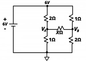
Example. A variation of the previous problem is shown in figure 3.34 where we want to consider the impact of different values of $x$ on the circuit. If we first consider the case where $x=\infty\Omega$ (meaning the resistor is an open circuit) then we would find via voltage-division analysis that $V_{A}=2V$ while $V_{B}=4V$ . Changing $x$ to a finite value, would result in current flow through $x$ owing to the voltage difference between $V_{A}$ and $V_{B}$ , and this would change the values of $V_{A}$ and $V_{B}$ . If $x=0\Omega$ (meaning the resistor is a short circuit) then we would have the upper $2\Omega$ and $1\Omega$ resistors in parallel, producing an equivalent resistance of $\frac{2\cdot1}{2+1}=\frac{2}{3}\Omega$ . Likewise, the lower resistors would be in parallel with an equivalent resistance of $\frac{2}{3}\Omega$ . In this case, $V_{A}=V_{B}=3V$ via voltage division. If resistance $x$ were some finite value other than $0$ , we would use node voltage analysis to determine $V_{A}$ and $V_{B}$ for this circuit.

Notice: we sometimes use lower-case variable names, such as $v_{A}$ and $i_{A}$ and other times we use capitalized or upper-case variable names, such as $V_{A}$ and $I_{A}$ . Why do we do this? The answer is convention: capitalized, or upper-case variables are, by convention, used to represent DC, or non-time varying voltages and currents in circuits. Lower-case variables are use for the more general case including both time varying and non-time varying, voltages and currents. When we derive expressions, we use lower-case variables for generality (ie, the results can apply to both AC and DC cases). When we work with specific examples of DC voltages and currents, we would then use the upper-case or capitalized variable names.

License

Icon for the Creative Commons Attribution 4.0 International License

Applied Electrical Engineering Fundamentals by David J. McLaughlin is licensed under a Creative Commons Attribution 4.0 International License, except where otherwise noted.

License

Share This Book