Weighting logarithmic data

Brokk Toggerson; Aidan Philbin

Weighting logarithmic data

Be careful weighting logarithmic data!

As discussed in the section Overview of Least Squares, the ordinary least squares method (OLS) does not take the uncertainties into account. In order to include this information, we normally weight each data point by its uncertainty:

We replace $x \rightarrow x \cdot \sigma_y$ and $y \rightarrow y \cdot \sigma_y$ .
We then plot $y \cdot \sigma_y$ vs. $x \cdot \sigma_y$ ,
Fit this new plot.
Use that slope.
Recalculate the intercept using the fact that the best fit line must pass through $( \bar{x}, \bar{y} )$ .

When looking at a plot involving logarithms, you may be inclined to follow the same procedure:

Instead of plotting $\log (x)$ vs. $\log (y)$ , you would probably plot $\log (x) \cdot \sigma_{\log (y)}$ vs. $\log (y) \cdot \sigma_{\log (y) }$ .
Fit this new plot.
Use that slope.
Recalculate the intercept using the fact that the best fit line must pass through $( \bar{\log (x)}, \bar{\log (y)} )$ .

Key Takeaways

This procedure is incorrect! To see why, we need to recall that for logarithms

$B \log (A) = \log \left( A^B \right)$
$\log (A) + \log(B) = \log(AB)$ .

This second property is key! It means that to weight the data, we should not multiply, but add!

The correct procedure is then:

Instead of plotting $\log (x)$ vs. $\log (y)$ , you should plot $\log (x) + \sigma_{\log (y)}$ vs. $\log (y) + \sigma_{\log (y) }$ .
Fit this new plot.
Use that slope.
Recalculate the intercept using the fact that the best fit line must pass through $( \bar{\log (x)}, \bar{\log (y)} )$ .

Examples

Dummy data

Consider the dummy data in the table below. These data were generated by adding noise to $y = x^{8/3}$ .

$x$	$\sigma_x$	$y$	$\sigma_y$
1.180499	0.131821	5.39407	0.418129
2.080013	0.133082	39.58304	6.400246
3.173837	0.243102	111.9454	26.41957
4.244258	0.447769	176.9608	29.47852
5.544937	0.518255	361.4891	36.77549
6.29372	0.679241	577.9257	124.7652
8.456563	0.733756	933.2456	81.81379

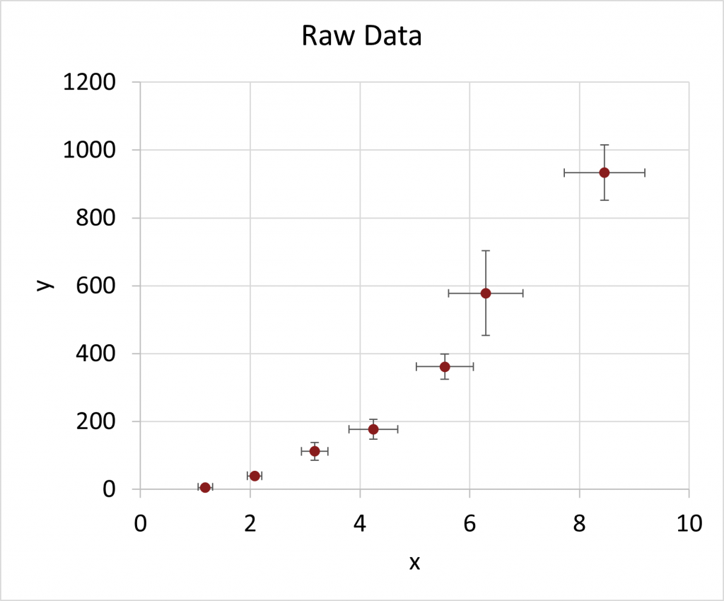
The graph of these data, which is obviously non-linear is shown below

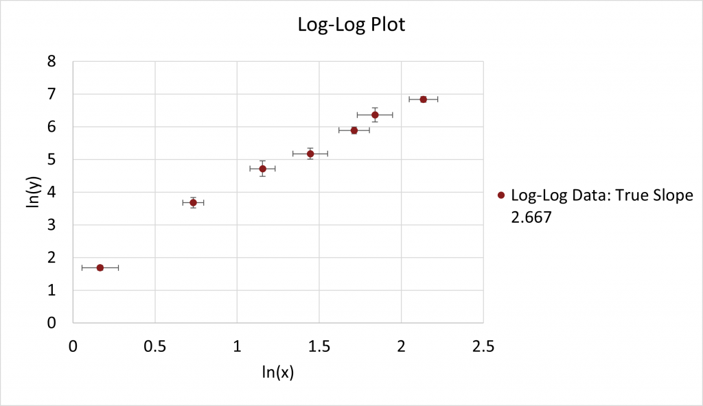
Linearize the Dummy Data Using Logarithms

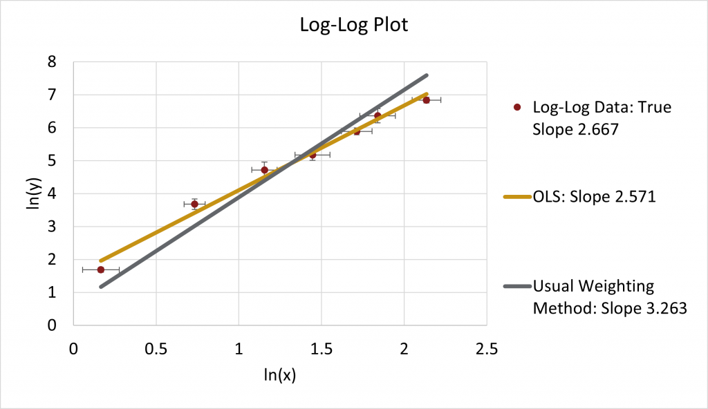
To linearize the data, we do a log-log plot. I will use log-base-e or natural logarithm $\ln$ . The result is, as expected, a straight line. The “correct” slope of this line should be $8/3 = 2.6\bar{6} \approx 2.667$ as that is the formula I used to make the data.

Do Our Usual Weighting Procedure

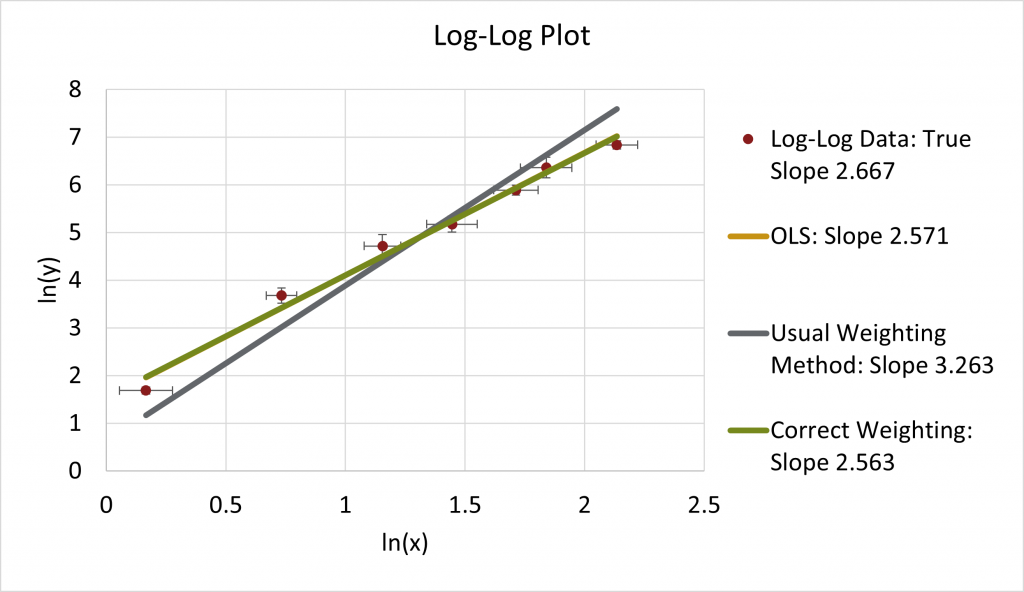
If we do our usual weighting procedure $\log (x) \cdot \sigma_{\log (y)}$ vs. $\log (y) \cdot \sigma_{\log (y) }$ , the result is a slope that is 3.263. This fit looks pretty bad, and the result is far from the “true” value.

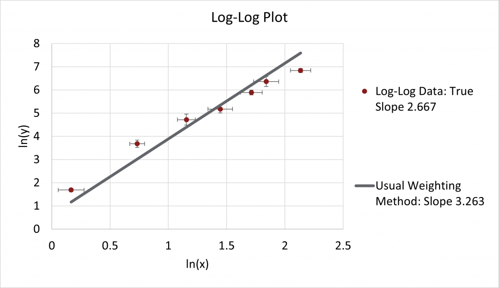
Usual weighting of noisy y=x^(8/3) data on a log log plot

This fit looks particularly bad when the default ordinary least squares fit, OLS, yields a slope of 2.571:

The OLS of the log-log y=x^(8/3) yields a slope of 2.571

Correct weighting

In contrast, the weighting done with addition: $\log (x) + \sigma_{\log (y)}$ vs. $\log (y) + \sigma_{\log (y) }$ yields a slope of 2.563, back in the correct range.

License

Icon for the Creative Commons Attribution-ShareAlike 4.0 International License

Physics 132 Lab Manual by Brokk Toggerson and Aidan Philbin is licensed under a Creative Commons Attribution-ShareAlike 4.0 International License, except where otherwise noted.