
Monte Carlo Error Propagation
Learning Objectives
How to apply the concepts of Monte Carlo to propagate errors.
Review of the assumptions of our data
Review of assumptions of the data that we are working under
-
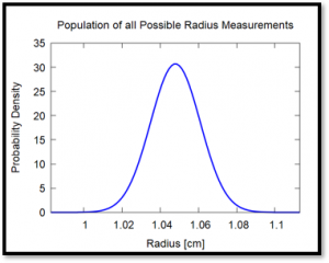
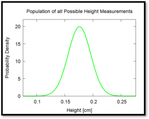
The set of the infinite number of possible measurements of a continuous variable like thickness will be a normal distribution.
-
Mean μ
-
Standard deviation σ
-
-
The mean
 of our sample of size N
![\[ \bar{x} = \frac{1}{N} \sum_i^N x_i \]](http://openbooks.library.umass.edu/p132-lab-manual/wp-content/ql-cache/quicklatex.com-3631977c3c20c79622f6b6056c7f6647_l3.png "Rendered by QuickLaTeX.com")
is a good estimate of the mean of the population μ.
-
The standard deviation of our sample
![\[ \sigma = \sqrt{ \frac{1}{N-1} \sum_i^N (x_i - \bar{x})^2 } \]](http://openbooks.library.umass.edu/p132-lab-manual/wp-content/ql-cache/quicklatex.com-ec7db37ae980c69982e2bcbd25a279a4_l3.png "Rendered by QuickLaTeX.com")
is a good estimate of the standard deviation of our population.
Below you can see our example data that we’ve been using throughout this lab: 10 measurements of radius and 10 measurements of the height or thickness. The mean and standard deviations previously calculated are also shown. We are assuming that these measurements are independent: that the thickness of the of the nickel and its radius are not correlated with each other in any way. For example, in observation number six, the radius is above the mean while the height is actually below the mean. This is what we mean when we say that they’re independent: just because the radius is high doesn’t necessarily mean that the thickness is also high.
| Observation | Radius [cm] | Height [cm] |
| 1 | 1.060 | 0.190 |
| 2 | 1.055 | 0.200 |
| 3 | 1.050 | 0.180 |
| 4 | 1.060 | 0.190 |
| 5 | 1.055 | 0.200 |
| 6 | 1.050 | 0.150 |
| 7 | 1.025 | 0.150 |
| 8 | 1.050 | 0.150 |
| 9 | 1.050 | 0.150 |
| 10 | 1.025 | 0.170 |
| Mean | 1.048 | 0.176 |
| Std. Dev. | 0.013 | 0.020 |
 |
 |
Principles of Monte Carlo Error propagation
In the case of our data
![\[ V = \pi r^2 h. \]](http://openbooks.library.umass.edu/p132-lab-manual/wp-content/ql-cache/quicklatex.com-65c0275da044af2a80148974f3a4b5b6_l3.png "Rendered by QuickLaTeX.com")
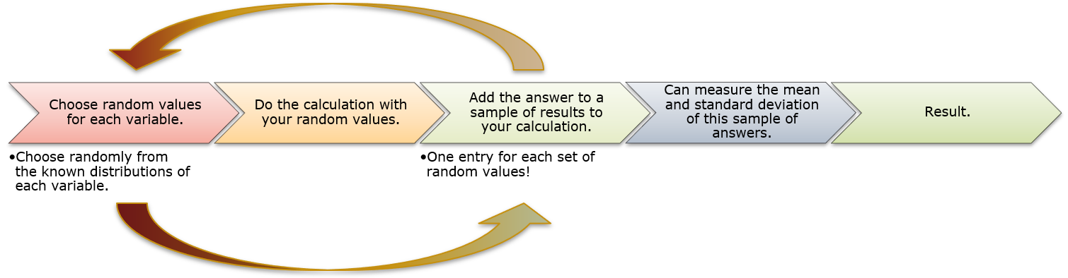
For each pair of height and radius, we’re going to get a volume and build up a sample of volumes. We’re going to repeat this a bunch of times and then we can measure the mean and standard deviation of this sample of volumes and that will give us our result.
Doing Monte Carlo error propagation “by hand”
- Take your measurements and write them on little scraps of paper: you should have 10 radii and 10 heights.
- Put them in a boxes (ideally with lids): one for radii and one for heights.
- Shake and pull out one radius and one thickness.
- Calculate volume.
- Put the radii and height back in their respective boxes.
- Repeat steps 1 – 5 ten times to get a sample of 10 volumes.
- Determine the mean and standard deviation of those results.
