
Introduction to Linearizing with Logarithms
Brokk Toggerson
Introduction
In a previous lab, you used algebra to linearize data: you just moved variables around to make something that wasn’t a line look like a line so that you could fit it. While this is a common way of linearizing data, a far more common approach is to use logarithms. Logarithms can also be used to linearize data and are seen throughout the literature in the form of log-lin plots, where instead of plotting y vs. x, one plots the logarithm of y vs x, and log-log plots, where the logarithm of y is plotted against the logarithm of x.
Log-Lin Plots
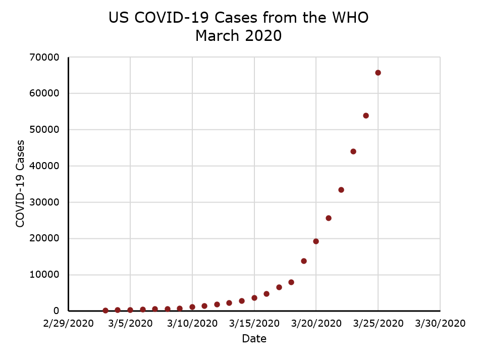
For example, when I plot the number of COVID-19 cases in the US in March 2020 according to the WHO, the result is an exponential looking curve.
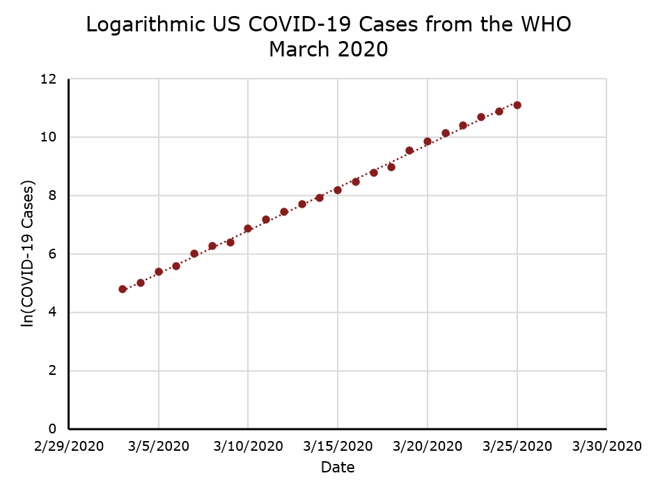
However, if I plot the natural logarithm (ln) of the number of cases on the vertical axis instead, the result is a straight line, and we know how to fit those!
Log-Log Plots
Another example is so-called Kleiber’s Law which is an empirical relationship between metabolic rate of organisms  and their mass

where  is a constant and
  is the power. Thommen et al [1] looked at this relationship in planarians (flatworms). The result is shown below along with an ordinary least fit line. You can see that the data are not exactly linear.
![Metablolic rate [uW] vs. planarian mass [mg] follows a non-linear relationship](http://openbooks.library.umass.edu/p132-lab-manual/wp-content/uploads/sites/26/2020/10/Thommen-et-al-Linear.png)
However, when, as is done in the paper, the data are plotted logarithmically, this time on both the horizontal and vertical axes, the result is a line.
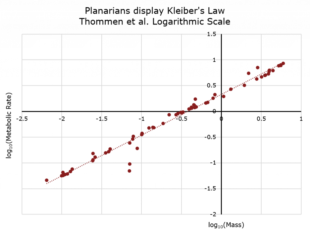
Due to the properties of logarithms (reviewed in a later section), the slope of this line is the power and the intercept is  . It turns out, for reasons not completely understood, that the power
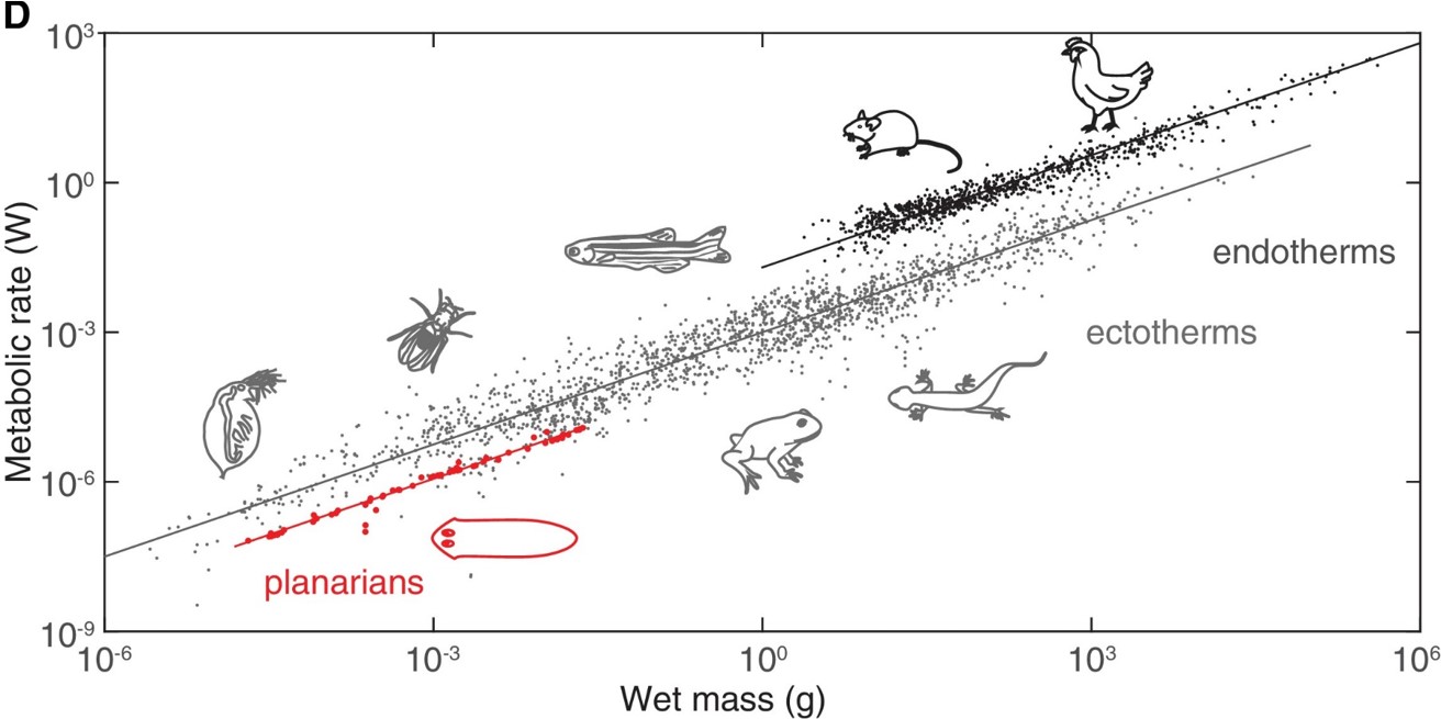
  for a large range of species from bacteria to humans as seen in their figure 1D shown below and described more in A. Makarieva et al [2].
Clearly logarithms are used extensively in the scientific literature to linearize data. This lab will explore how to use logarithms to understand more complex data.
- Thommen, Albert, Steffen Werner, Olga Frank, Jenny Philipp, Oskar Knittelfelder, Yihui Quek, Karim Fahmy, et al. “Body Size-Dependent Energy Storage Causes Kleiber’s Law Scaling of the Metabolic Rate in Planarians.” eLife. eLife Sciences Publications Limited, January 4, 2019. https://doi.org/10.7554/eLife.38187. ↵
- Makarieva, Anastassia M., Victor G. Gorshkov, Bai-Lian Li, Steven L. Chown, Peter B. Reich, and Valery M. Gavrilov. “Mean Mass-Specific Metabolic Rates Are Strikingly Similar across Life’s Major Domains: Evidence for Life’s Metabolic Optimum.” Proceedings of the National Academy of Sciences 105, no. 44 (November 4, 2008): 16994–99. https://doi.org/10.1073/pnas.0802148105. ↵
