
Introduction to Monte Carlo Methods
Learning Objectives
This section will introduce the ideas behind what are known as Monte Carlo methods.
Motivation and a bit of history

There are some problems in science that are so complicated that they just can’t be analyzed by formulas that you can write down on a piece of paper. This is particularly true in biology and health sciences because the problems are so complex. One example is the folding and shape of proteins. This is famously a very difficult problem. How do you solve such problems? Well, one technique is to use probability, random numbers, and computation. These methods are known as Monte Carlo methods. They are named after the town of Monte Carlo in the country of Monaco, which is a tiny little country on the coast of France which is famous for its casinos, hence the name. These methods rely on computers to simulate the results and these were first really used in the Manhattan project in a serious way. Now, however, they are used in all fields: understand systems like:
- Understanding systems: cost overruns or time overruns.
- Finance: predicting if a commodity price is going to go up or down.
- Resource exploration: oil and other minerals
All of these different fields use Monte Carlo methods to gain a deeper understanding of complex problems.
A first example – calculating π
As a first example of how Monte Carlo methods work, we’re going to do something maybe a little silly and calculate  . To see how we can do this using Monte Carlo:
- Consider a square that’s one meter on a side. Call the horizontal direction x and the vertical direction y.

A square 1m on a side - Inside the square, let’s put a circle. Since the circle is 1 m in diameter, it has a radius of half a meter.
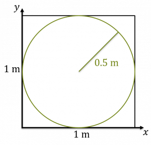
A circle of diameter 1 m inside a 1m square. - Now, the area of the circle divided by the area of the square is
![\[ \frac{A_{circle}}{A_{square}} = \frac{\pi r^2}{s^2}. \]](http://openbooks.library.umass.edu/p132-lab-manual/wp-content/ql-cache/quicklatex.com-3a1dcb1dcc2399d64a2e326add57024e_l3.png "Rendered by QuickLaTeX.com")
In our case, the radius is 0.5m and the side is 1m, so the ratio of areas is
![\[ \frac{A_{circle}}{A_{square}} = \frac{\pi (0.5)^2}{(1)^2}. \]](http://openbooks.library.umass.edu/p132-lab-manual/wp-content/ql-cache/quicklatex.com-133c02981be415295f7b852004fd10a4_l3.png "Rendered by QuickLaTeX.com")
Which, when you simplify it is
![\[ \frac{A_{circle}}{A_{square}} = \frac{\pi}{4}. \]](http://openbooks.library.umass.edu/p132-lab-manual/wp-content/ql-cache/quicklatex.com-e6d580b30a0399bba4b2b5fabc162aa8_l3.png "Rendered by QuickLaTeX.com")
- Now, we throw a dart (or in a computer, we choose a random x and y value each between 0 and 1). Let’s say that for this first dart, we get a very large x and a very small y, so the dart lands in the outer corner. We then check to see is the dart inside the circle. Obviously, if you’re doing physical darts you can actually see, but if you’re doing calculation well you would check to see if
![\[ \sqrt{x^2 + y^2} < 0.5. \]](http://openbooks.library.umass.edu/p132-lab-manual/wp-content/ql-cache/quicklatex.com-4b23d71912016f804efc0b9eccb36d25_l3.png "Rendered by QuickLaTeX.com")
If that is the case, then the dart is inside the circle. We now have one dart thrown and none inside the circle.
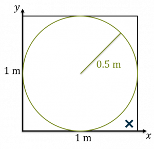
A dart thrown at our circle inscribed in a square. The dart lands outside the circle, but inside the square. Darts thrown Darts inside circle 1 0 - Now, throw another dart and repeat the process. Let’s say this dart lands inside the circle. As a result, we now have two darts thrown and one inside.
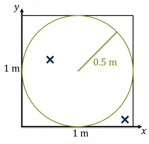
A second dart thrown at the circle inscribed in a square. This one lands inside the circle. Darts thrown Darts inside circle 2 1 - If you do a bunch of darts, the number of darts inside divided by the number outside will be the area of the circle divided by the area of the square. Think about it in terms of probability: you’re throwing darts at random
the number of darts that landed in the circle divided by the number of darts that land in the square is going to be the ratio of their areas. As we have already seen, this ratio is . If you do this for a bunch of darts, a bunch of dots in a computer, once you get to a couple hundred thousand you start to get a relatively reasonable approximation for .
Summary of calculating with Monte Carlo
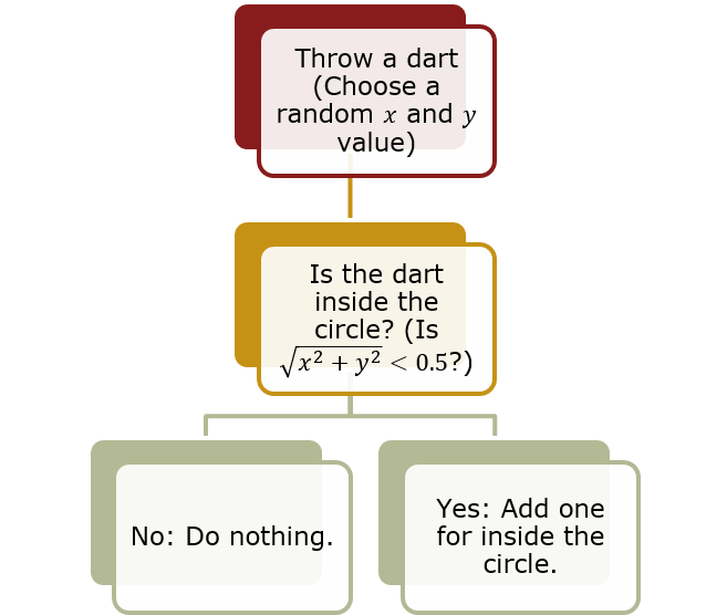
- Throw a dart (Choose a random x and y value)
- Check to see if the dart is inside the circle: (
 ?
?
- If no: just increment the number of darts
- If yes: increment the number of darts and the number of darts that land inside the circle.
- After enough darts, the ratio of inside to outside will be .
A biologically authentic example – protein folding
Folding proteins, is as described earlier, a famously difficult problem. Now, we will go through how you can use Monte Carlo methods to solve protein folding. The example I’m going to go through here is a simplified version of the method described in Earl et al.[1].
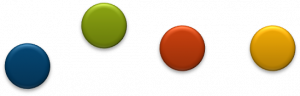
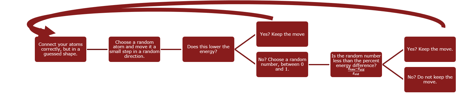
- To start, you correctly connect your atoms in some random guessed shape. A straight line will even work, but if you can make a better guess, the computation will take less time.

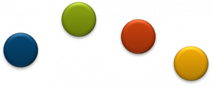
We will explore a toy protein of only four atoms. - Choose a random atom and move it a small step in a random direction. In our case, I’m going to move the second green atom just up and to the right just a little bit.

Choosing the second green atom at random, lets move it a small random distance in a random direction: up and to the right. - Now go and calculate the energy in this configuration.
- Is the new energy lower than the energy you started with?
- If the answer is yes (and let’s assume it is), leave the green atom where it is and start over choosing a different atom.
- Now we’re going to go back to step 2 and choose a different random atom, say the the first blue atom, and move it a small random distance in a random direction: let’s say down and to the right.
As the second step, move the first blue atom down and to the right. - Now go and calculate the energy in this configuration.
- Is the new energy lower than the energy you started with?
- If the answer is no (and let’s assume it is), calculate the percent change in energy:
 . Note this number will be between 0 and 1 because our steps are so small.
 - Choose a random number between 0 and 1.
- If the random number is less than the percent change in energy (which let’s assume is the case), keep the move anyway. The reason for keeping small increases in energy are local minima: we are looking for the smallest possible energy configuration. However, there may be configurations that represent smaller energy configurations, but not the overall smallest. For a graphical depiction consider the graph below, the first dip is a local minimum, but we want to find the smallest minimum which is the second one. Keeping slightly larger changes in energy, helps us avoid getting stuck in these smaller, but not smallest, energy configurations.
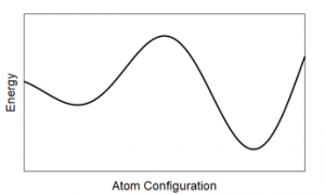
The first dip is a local minima, but we want the global minimum which is further to the right.
- Go back to step 2. This time, we will randomly choose the the last yellow atom to move a random amount in a random direction, in this case is down and to the left.
As a next step move the yellow atom down and to the left. - Now go and calculate the energy in this configuration.
- Is the new energy lower than the energy you started with?
- If the answer is no (and let’s assume it is), calculate the percent change in energy: . Note this number will be between 0 and 1 because our steps are so small.
- Choose a random number between 0 and 1.
- This time, let’s say the random number is larger than the percent change. In this case, reject the move and put the yellow atom back.
We return the yellow atom back to where it was.
- Repeat this hundreds and hundreds and hundreds and hundreds of times and, it may seem weird but, you actually can end up with the correct answer!
Graphical Representation of the Monte Carlo method for protein folding
Below, you can see this method in action. You can see that this is a Monte Carlo simulation of a polypeptide chain and the author starts with all the atoms in basically a straight line and then runs the simulation. You can see they’re jiggling around at random. As each atom randomly moves, the computer is calculating the energy and leaving the atoms if the energy is lower and sometimes even if it is higher. Run this run for hundreds of thousands of computations and ultimately it settles down into what is actually the correct answer for this polypeptide chain!
Summary
Key Takeaways
-
Monte Carlo (MC) methods use random numbers to solve problems that cannot be solved any other way.
-
Used in a variety of fields:
-
Physics.
-
Biology.
-
Geosciences.
-
Finance.
-
…
-
-
In this lab, you will use a MC method to propagate uncertainties.
- Earl et. al. Monte Carlo Simulation. Molecular Modeling of Proteins pp 25-36. Retrieved August 26, 217 from: https://link.springer.com/protocol/10.1007/978-1-59745-177-2_2 ↵
