
Linearizing Data with Algebra
Plotting strange combinations of variables
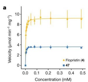
As described in the Introduction to this lab, while many relationships in nature are linear, many others are not. However, as discussed in a prior lab, linear fits have the advantage that they are easy for our ape-brains to comprehend. Moreover, the fit to a line only has two parameters: the slope and the intercept which makes it easy to understand how the fit is done in terms of the residuals etc. Can we use the benefits of linear fits for non-linear data? The answer (of course given the title of this lab), is yes! One way to do this is by simply plotting combinations of variables on each axis instead of simple things like time or distance. For example in figure 3a from Q. Li et al.[1] we see  plotted on the vertical axis. Sometimes, by choosing the correct set of axes, you can make data that is not a line into a line.
Example from Quantum Mechanics and Chemistry with which you should be familiar
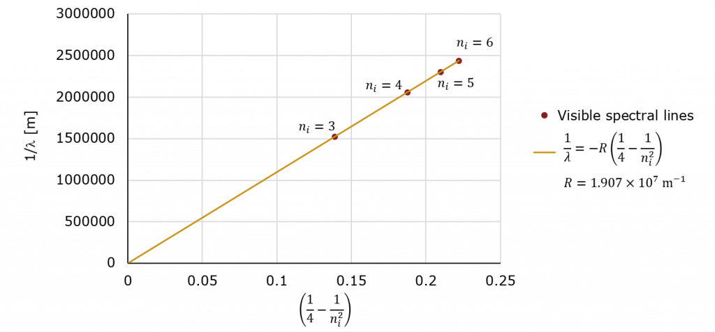
In Chemistry and our Unit on Quantum Mechanics, we discussed the atomic spectrum of hydrogen the visible spectral lines of which (the so-called Balmer series) are shown below.

We solved for these wavelengths using conservation of energy:


For hydrogen, the energy levels are given by  while the energy of the photon
  is given by the familiar formula
  . The result is

For the visible lines,  is always equal to 2 leaving us with


Dividing across by  we have

While this may not look like it, it is the equation for a line! All we need to do is plot  (which is unit-less) on the horizontal and
  on the vertical (in units of 1/m) and the slope will be
  with an intercept of zero!
Key Takeaways
Sometimes, by plotting seemingly strange combinations of variables you can convert a non-linear relationship into a linear one!
- Li, Qi, Jenna Pellegrino, D. John Lee, Arthur A. Tran, Hector A. Chaires, Ruoxi Wang, Jesslyn E. Park, et al. “Synthetic Group A Streptogramin Antibiotics That Overcome Vat Resistance.” Nature 586, no. 7827 (October 2020): 145–50. https://doi.org/10.1038/s41586-020-2761-3 . ↵
