Finding Mean and Standard Deviation in Google Sheets

Now we need to find the mean and standard deviation of our height and radius values. We’ll use Google Sheets to do this.

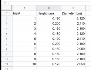
Below is an example of data collected for this lab. I have a column for trials one through ten, along with columns for corresponding nickel heights and diameters.

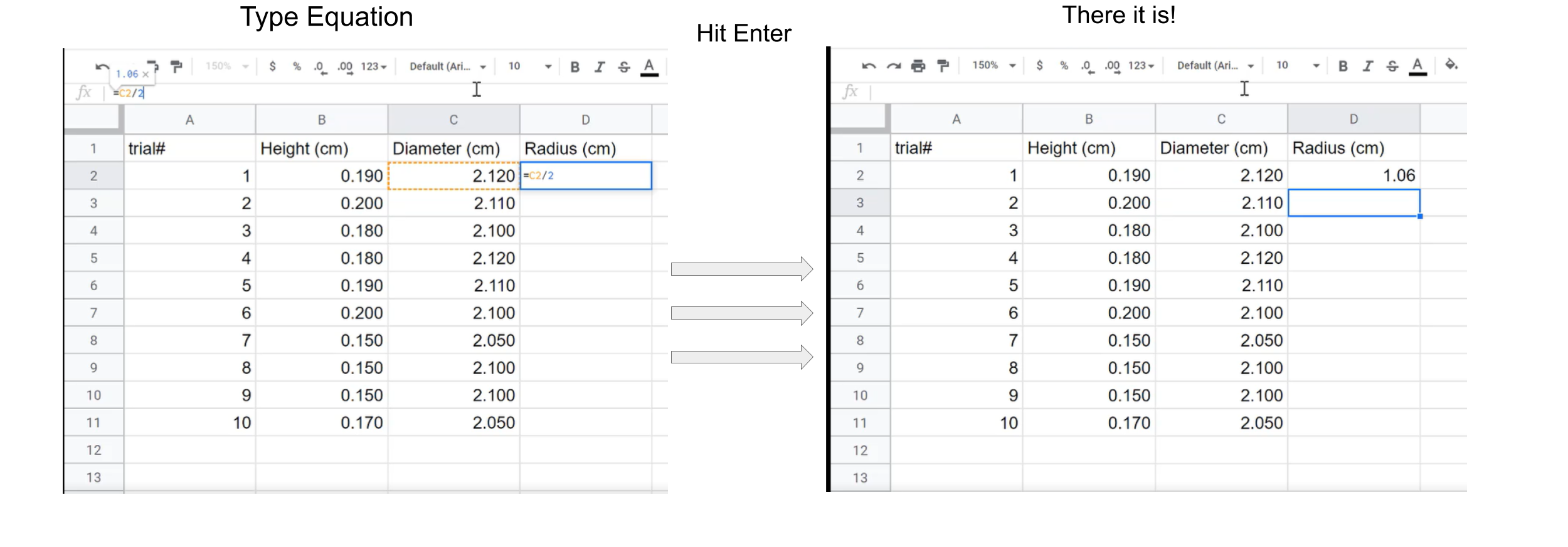
What we are looking for first is the mean value for height and the mean value for radius. It is immediately apparent that we do not have values for radii. We do know that the diameter is twice as long as the radius, so we can divide our diameter data by 2 to get radii. We’ll make a column next to Diameter and input the respective radius for each trial. Because we are using a spreadsheet program, we will not have to type in any of the diameters again, instead we can just click on the cell we have them in. We’ll type in the equation for radius, and let Google Sheets solve it. To type in this the equation, click the cell corresponding to the radius for trial 1.  In the fx line, type an equals sign “=”, click on the first diameter (cell C2 here), then “/2”. This will return the first radius value.

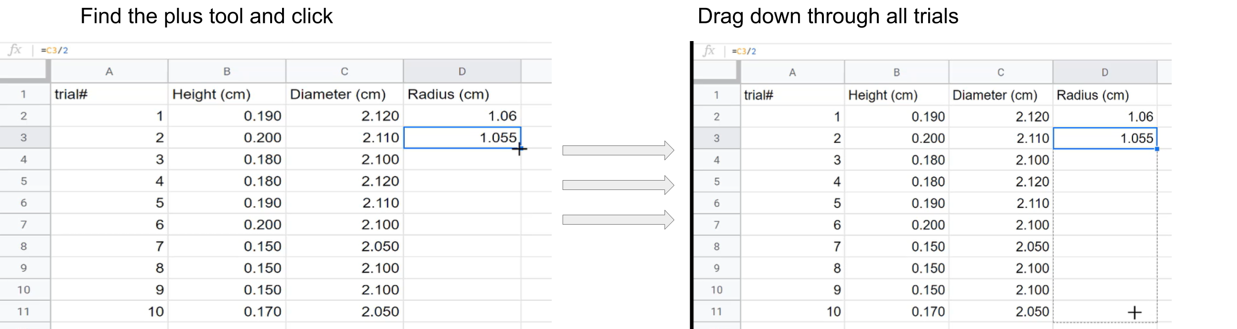
Each trial will have a radius corresponding to the respective diameter. For the second radius, we’ll type “=C3/2” in cell D3. This is nice, we don’t even have to solve the equation ourselves! Yet, there is one more trick that will make this process even easier. The Fill Tool, or Plus Tool as I like to call it, pops up when you click a cell and mouse over its bottom right corner. This tool will allow us to type the equation only once, then we can drag the plus tool to copy the equation to another cell. We already have equations in cells D2 and D3, they correspond to our first two radii. With the plus tool at the bottom right corner of cell D3, we can click and drag the plus down to cell D11, our last radius.

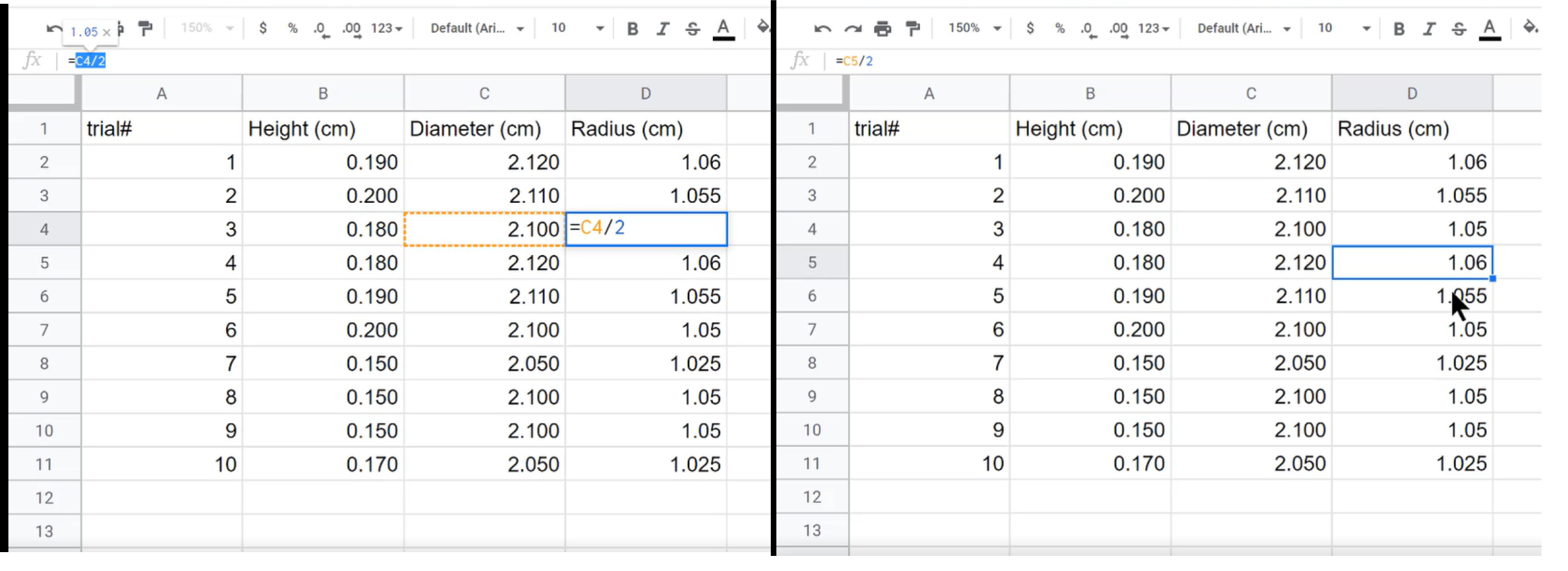
Clicking on cells D4 and D5, we see that D4=C4/2 and D5=C5/2. Google Sheets knows that our equation changes for each trial, and thus it uses the right diameter each time.

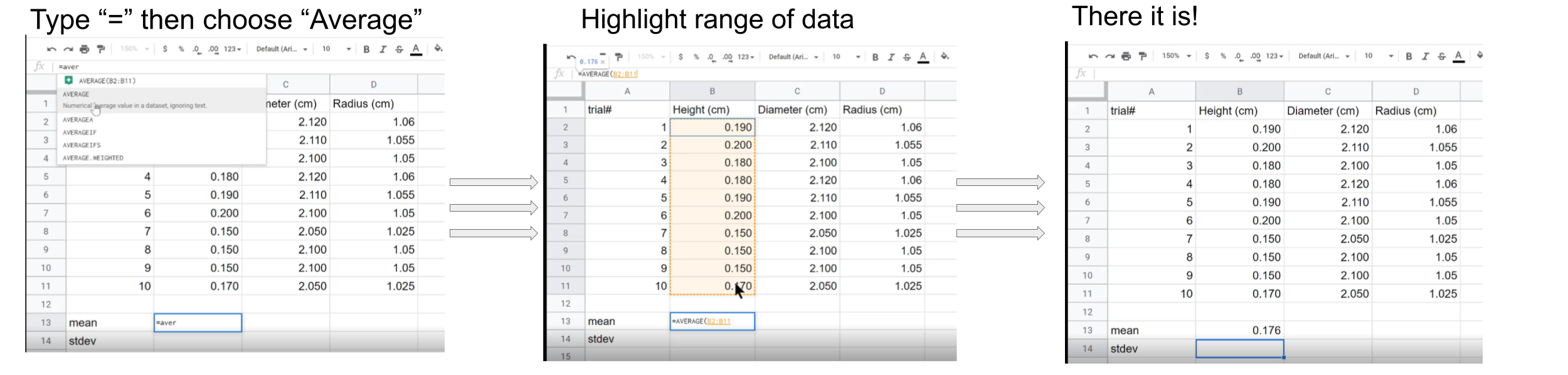
Finally now, we have the heights and radii for each trial and we can move on to finding the means and standard deviations. We’ll use row 13 for the means and a row 14 for the standard deviations. To calculate these two values for all three of our columns, we’ll use some spreadsheet functions. Functions are like equations, they have to start with an “=” sign, but instead of typing out the equation, we type in the name of the function, and then we enter the arguments – inputs – for the function. Both the Average function and the Standard Deviation function take ranges of data as their arguments. This makes sense, as we are trying to find means and standard deviations for data we collected with ten trials.

Just as the plus tool works for replicating equations, it replicates functions too. We can click the plus tool in cell B13, and drag it over to cell D13, and then we’ll have the mean for height, diameter, and radius.

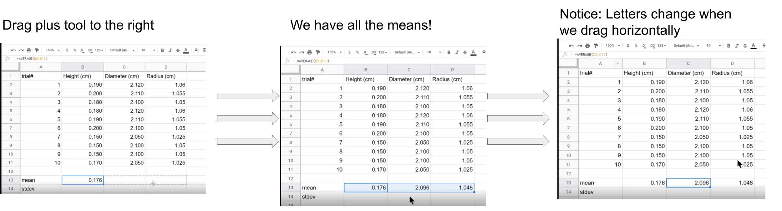
When we use the plus tool to drag an equation or function vertically, the cell number will increment for the change in row. When we use the plus tool to drag an equation or function horizontally, the cell letter will increment for the change in column.

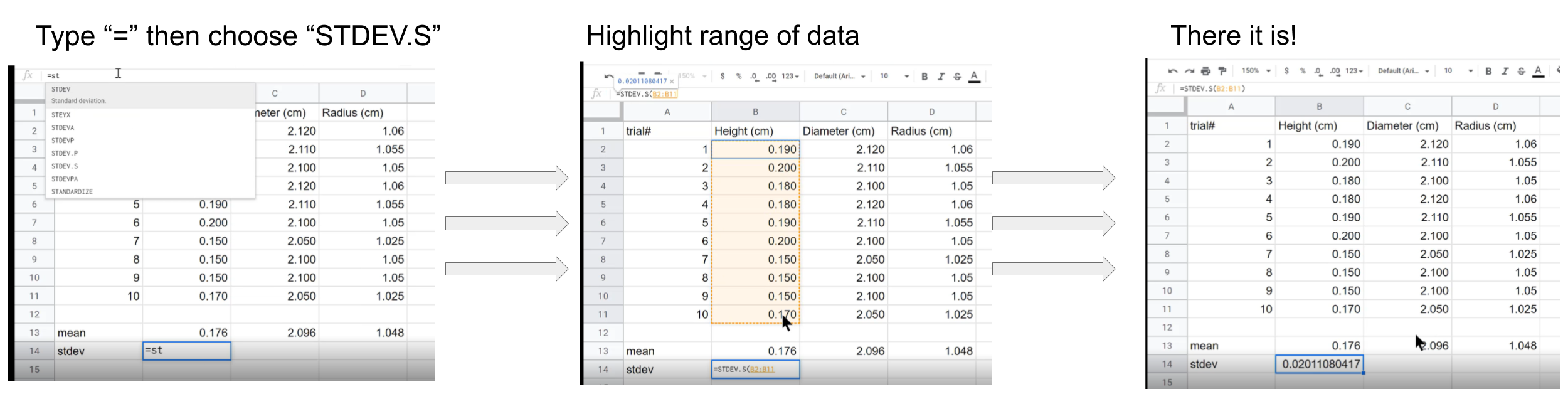
Now we can find standard deviation with another function. There are actually a lot of different standard deviation functions built into Google Sheets. We have a measurements on a 10-nickel sample of a population of all nickels, so we’ll use STDEV.S, this function returns the standard deviation of a sample.

Now we can drag the plus tool – just as we did with the means – to find all three standard deviations.

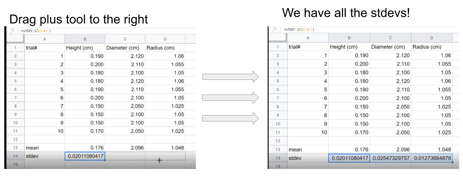
Now we have all our means and our standard deviations!