The simulation above, provided by PhET is about probability. Click the “Lab” and explore along.

What this is is a plinko-board.  If I drop a ball, you can see it goes bouncing down the board, and ends up in one of the bins at the bottom. Now, increase the impact by making as many rows as possible: 26. The slider below shows you that the probability of a ball going left or right when it hits a peg is 50/50, i.e. half the time the ball bounces left and half the time the ball bounces right. Now, click the several balls option near the top and see what happens. As the balls begin to hit the bottom and fill the bins, at first it seems kind of a random mess. As time goes on, however, we see a particular shape beginning to form we see a shape known as a bell curve, normal distribution, or a Gaussian, and with more and more spheres they begin to fill the pattern out. You can click on “Ideal” to see the ideal shape. The result is not perfect, but if you let this keep running to about 500 balls or so it will begin to fill this shape out quite nicely.

Now, let’s see what happens when it’s not a 50/50 when the ball hits a peg let’s make it like a 30/70 split by moving the slider to the left until it says “30.” What this means is, as the ball falls 30 percent of the time it will go right and 70 of the time it will go left. Drop a single ball and see what happens. Now, drop a lot of balls. Again, at first the result seems random, but as time progresses, lo-and-behold, once again we begin to fill out the same bell curve. The only difference is that the bell curve is shifted to the left. So we don’t need a 50 50 probability to get this shape. A 30/70 split over-and-over achieves the same result. This is an example of what is known as the central limit theorem.

The Normal Distribution

Properties of the normal distribution

Below is a normal probability distribution. We can see the variable on the horizontal axis. In this case, we are thinking about a continuous variable like the dropping ball from the section on uncertainty. On the vertical axis, we have what’s known as probability density, which we will return to in in a moment. As a probability distribution, the area under this curve is defined to be one.

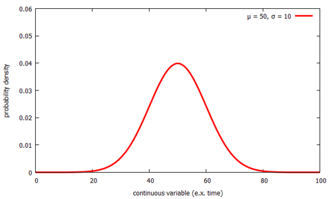
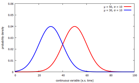
The normal distribution is characterized by two numbers μ and σ. The symbol μ represents the the central location. Below we see two normal distributions. The one above, with μ = 50 and another, in blue, with a μ = 30. As you can see, it just shifts the distribution to the left to be centered on 30 instead of being centered on 50.

The other important variable, σ, represents the width of the distribution. Below we add a third normal distribution, in black, which also has μ = 50, but now has σ = 7 instead of σ = 10 like the other two curves. You can see the result is skinnier. However, if the area underneath the normal distribution must always be equal to 1, then in order to make it skinnier, it must also get it taller.

Probability density and the area under the normal distribution

What is meant by the vertical axis: probability density? It means that the probability of a measurement falling within a particular range is given by the area under the curve (integral in calculus language) corresponding to that range. In the figure below, the range from 50 to 60 is shaded. This region visually represents the probability of a measurement falling between 50 and 60. Now you can see why the area underneath the entire curve must be one: the probability of something happening must be 100%.

Formula of the normal distribution (Optional)

You will not be working with the formula of the normal distribution explicitly too much in this course, but if you are curious, it is

It is somewhat ugly, but you can see it depends upon the central location μ, and the width σ. The x is then our variable on the horizontal axis. The thing out front ensures that the area underneath is in fact equal to 1.

Interpreting the Normal Distribution and Standard Deviation

What is standard deviation?

So, you’ve probably guessed that μ is the mean of your data, but what is σ? We know it’s the width of our distribution, but how is it connected to our data? The answer is σ  is the standard deviation of your data, and it describes how spread out your data are: is it a wide fat distribution or a narrow skinny one.

If you have a sample from some population,  you calculate the standard deviation using the formula below:

which is super ugly so we’ll go through it piece by piece to understand how this formula works:

1. For each data point x_i, you subtract it from the mean μ (so you have to calculate the mean first!).
2. You then square each result. Squaring serves the important function of making all the terms positive meaning that data points that happen to be above the mean can’t cancel out points that are below the mean.
3. Take all these answers and add them up.
4. Divide by the size of the sample N minus 1.
5. Take the square root of the answer.

Technically, this is called the corrected sample standard deviation although you don’t need to know that term but you might have seen it in a statistics course. The corrected sample standard deviation is often assumed to be a good estimate of the standard deviation of the population although there are specific conditions that must be met for that assumption to be true. More importantly, it provides a measure of the statistical uncertainty in your data.

Standard deviation and the area under the normal distribution

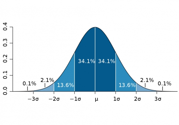
Now let’s come back to the ideas of area and probability. Recall the area under the curve is the probability. One nice feature of the normal distribution is that, in terms of σ, the areas are always constant. Below we see a normal distribution. We can expect a measurement to be within one standard deviation of the mean about 68% of the time. It doesn’t matter how much I stretch this distribution or squeeze it down, the area between -1σ and +1σ is always going to be about 68%. We can expect a measurement to be within two standard deviations of the mean about 95% of the time and within three standard deviations 99.7% of the time. These are really good numbers to have in your head as many research papers that you might read you will see discussion of “one sigma,” “two sigma,” or “three sigma” effects.

How to write numbers in this class

As you will see in the examples below, I keep all numbers during the calculation. YOU TOO SHOULD DO THIS! DO NOT ROUND IN THE MIDDLE! Round only at the end.

How should you round? Use your uncertainty to determine how many digits to keep (as opposed to significant figures rules, hopefully this lab will show you why!). Keep one digit of your standard deviation and round your mean to that same number of digits. We are using the data itself to determine how many digits to keep instead of the significant figures rules.

Examples

Let’s do an example going through all this information using the same falling ball example we used in Introduction to Statistical vs. Systematic Uncertainty. Below are the observations from my watch (remember they bounced
around π) and your watch.

Observation	My Watch [s]	Your Watch [s]
1	3.142	5.312
2	3.140	5.002
3	3.145	5.687
4	3.143	5.479

Calculating standard deviation

The results of the steps are in the table below.

1. Calculate the mean by adding up all four numbers and dividing by four to get 3.143s
2. For each value determine the difference from the mean. For the first value, we get 3.142 – 3.143 = -0.001s. Repeat this for all subsequent values.
3. Square each result. For the first value . Repeat this for all subsequent values.
4. Add these squared differences to get .
5. Divide by to get .
6. Take the square root to get the standard deviation of 0.00208s.

Observation	My watch [s]	Difference from the mean [s]	Difference from mean squared [s2]
1	3.142	-0.001
2	3.140	-0.002
3	3.145	+0.002
4	3.143	0.000
		Sum
		Sum/(N-1)
		Standard Deviation	0.00208s

Writing your numbers

For my watch we got , while for your watch you should get . For my watch the uncertainty is in the milliseconds. I therefore round to that place and write my number as . For your watch, in comparison, the uncertainty is in the tenths of a second place. The number is then more exactly written as . You will notice that the significant figures rules would have told you to keep the same number of digits (three after the decimal) for both of these results. However, that is somewhat misleading for your watch: we do not know the precision of your watch to that level.

Understanding your Number

The result from my watch is where the uncertainty is now the standard deviation. If we use the usual normality assumption, what how often will my watch read a value in the range of 3.141s – 3.145s?

Since that range corresponds to one standard deviation, we expect my watch to give a result in that range about 68% of the time. This, of course, means that 32% of the time (1 time in 3!) my watch will give a value outside of this range!