
21 Vector Review

Instructor’s Note
You should already be familiar with vectors, but we will use them in this unit, so this chapter from Physics 131 is a review. If this material is familiar, feel free to go to the homework problems at the end (there are none embedded in the sections, as it is review).
Your Quiz would Cover:
- A vector is a quantity with a magnitude and direction
- Converting between magnitude/direction and the component form for any vector. This ties into the Pythagorean Theorem
Kinematics in Two Dimensions: An Introduction

Two-Dimensional Motion: Walking in a City
Suppose you want to walk from one point to another in a city with uniform square blocks, as pictured in Figure 2.
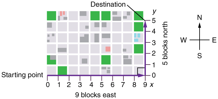
The straight-line path that a helicopter might fly is blocked to you as a pedestrian, and so you are forced to take a two-dimensional path, such as the one shown. You walk 14 blocks in all, 9 east, followed by 5 north. What is the straight-line distance?
An old adage states that the shortest distance between two points is a straight line. The two legs of the trip and the straight-line path form a right triangle, and so the Pythagorean theorem,  , can be used to find the straight-line distance.
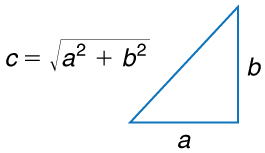 . This can be rewritten, solving for c :
Instructor’s Note
We will be using the Pythagorean theorem all throughout two-dimensional kinematics, as well as throughout this entire course. If you are uncomfortable or unfamiliar with the Pythagorean theorem, or even if it’s just been a long time since you’ve used it, please come see your instructor as soon as possible, and they will get you up to speed.
The hypotenuse of the triangle is the straight-line path, and so in this case its length in units of city blocks is  , considerably shorter than the 14 blocks you walked. (Note that we are using three significant figures in the answer. Although it appears that “9” and “5” have only one significant digit, they are discrete numbers. In this case, “9 blocks” is the same as “9.0 or 9.00 blocks.” We have decided to use three significant figures in the answer in order to show the result more precisely.)
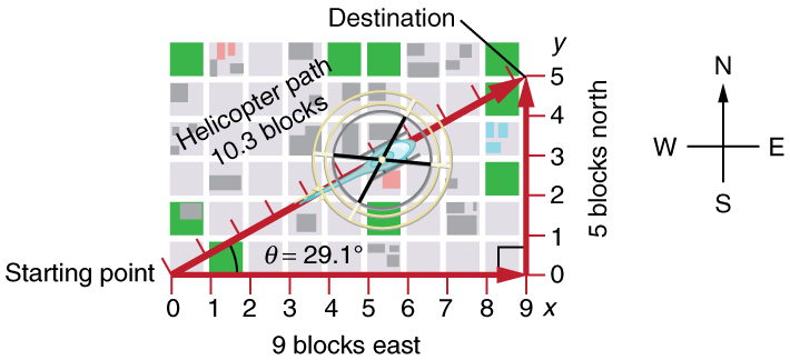
The fact that the straight-line distance (10.3 blocks) in Figure 4 is less than the total distance walked (14 blocks) is one example of a general characteristic of vectors. (Recall that vectors are quantities that have both magnitude and direction.)
As for one-dimensional kinematics, we use arrows to represent vectors. The length of the arrow is proportional to the vector’s magnitude. The arrow’s length is indicated by hash marks in Figure 2 and Figure 4. The arrow points in the same direction as the vector. For two-dimensional motion, the path of an object can be represented with three vectors: one vector shows the straight-line path between the initial and final points of the motion, one vector shows the horizontal component of the motion, and one vector shows the vertical component of the motion. The horizontal and vertical components of the motion add together to give the straight-line path. For example, observe the three vectors in Figure 4. The first represents a 9-block displacement east. The second represents a 5-block displacement north. These vectors are added to give the third vector, with a 10.3-block total displacement. The third vector is the straight-line path between the two points. Note that in this example, the vectors we are adding are perpendicular to each other and thus form a right triangle. This means we can use the Pythagorean theorem to calculate the magnitude of the total displacement. (Note that we cannot use the Pythagorean theorem to add vectors that are not perpendicular. We will develop techniques for adding vectors having any direction, not just those perpendicular to one another, in Vector Addition and Subtraction: Graphical Methods and Vector Addition and Subtraction: Analytical Methods.)
The Independence of Perpendicular Motions
Instructor’s Note
The idea of the independence of perpendicular motion is a fundamental one that you should take some time to think about, and there are some questions about this topic on the homework.
The person taking the path shown in the figure walks east and then north (two perpendicular directions). How far he or she walks east is only affected by his or her motion eastward. Similarly, how far he or she walks north is only affected by his or her motion northward.
Independence of Motion
The horizontal and vertical components of two-dimensional motion are independent of each other. Any motion in the horizontal direction does not affect motion in the vertical direction, and vice versa.
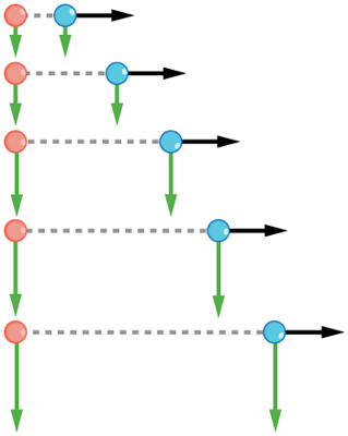
This is true in a simple scenario like that of walking in one direction first, followed by another. It is also true of more complicated motions involving movement in two directions at once. For example, let’s compare the motions of two baseballs. One baseball is dropped from rest. At the same instant, another is thrown horizontally from the same height and follows a curved path. A stroboscope has captured the positions of the balls at fixed time intervals as they fall.
Instructor’s Note
This graphic displays this concept quite nicely; notice how both balls fall downward at the same speed at each point, even though one of the balls has a horizontal velocity. Basically, the velocity of the ball in the x-direction has no effect on the velocity in the y-direction, and vice versa. This idea will be important, especially when working with vectors.
It is remarkable that for each flash of the strobe, the vertical positions of the two balls are the same. This similarity implies that the vertical motion is independent of whether or not the ball is moving horizontally. (Assuming no air resistance, the vertical motion of a falling object is influenced by gravity only, and not by any horizontal forces.) Careful examination of the ball thrown horizontally shows that it travels the same horizontal distance between flashes. This is due to the fact that there are no additional forces on the ball in the horizontal direction after it is thrown. This result means that the horizontal velocity is constant, and it is affected neither by vertical motion nor by gravity (which is vertical). Note that this case is true only for ideal conditions. In the real world, air resistance will affect the speed of the balls in both directions.
The two-dimensional curved path of the horizontally thrown ball is composed of two independent one-dimensional motions (horizontal and vertical). The key to analyzing such motion, called projectile motion, is to resolve (break) it into motions along perpendicular directions. Resolving two-dimensional motion into perpendicular components is possible because the components are independent. We shall see how to resolve vectors in Vector Addition and Subtraction: Graphical Methods and Vector Addition and Subtraction: Analytical Methods. We will find such techniques to be useful in many areas of physics.
Section Summary
- The shortest path between any two points is a straight line. In two dimensions, this path can be represented by a vector with horizontal and vertical components.
- The horizontal and vertical components of a vector are independent of one another. Motion in the horizontal direction does not affect motion in the vertical direction, and vice versa.
Vector Addition and Subtraction: Graphical Methods
Instructor’s Note
Your Quiz would Cover:
- Given two graphical representations of vectors, be able to draw the sum or difference. There are some simple procedures to follow. Solidify your understanding of these procedures, and we can work on why this makes sense in class.
- Describe both visually and mathematically what happens when a scalar is multiplied by a vector. If I give you a vector and a number, you should be able to turn the crank and multiply them mathematically. I am NOT expecting you to be able to do this graphically and will not ask you what it means. Just focus on the mechanics of how to do it.
- Convert between magnitude/direction and component form for any vector.
Vectors in Two Dimensions
A vector is a quantity that has magnitude and direction. Displacement, velocity, acceleration, and force, for example, are all vectors. In one-dimensional, or straight-line, motion, the direction of a vector can be given simply by a plus or minus sign. In two dimensions (2-d), however, we specify the direction of a vector relative to some reference frame (i.e., coordinate system), using an arrow having length proportional to the vector’s magnitude and pointing in the direction of the vector.
Figure 2 shows such a graphical representation of a vector, using as an example the total displacement for the person walking in a city considered in Kinematics in Two Dimensions: An Introduction. We shall use the notation that a boldface symbol, such as  , stands for a vector. Its magnitude is represented by the symbol in italics,
  , and its direction by
Instructor’s Note
It would be useful to pay attention to the notation in the following box.
Vectors in this Text
In this text, we will represent a vector with a boldface variable. For example, we will represent the quantity force with the vector  , which has both magnitude and direction. The magnitude of the vector will be represented by a variable in italics, such as
  , and the direction of the variable will be given by an angle .
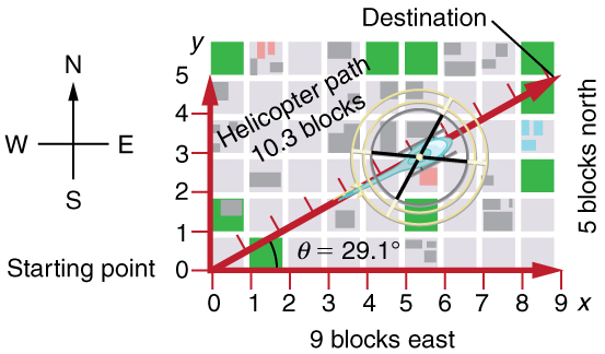
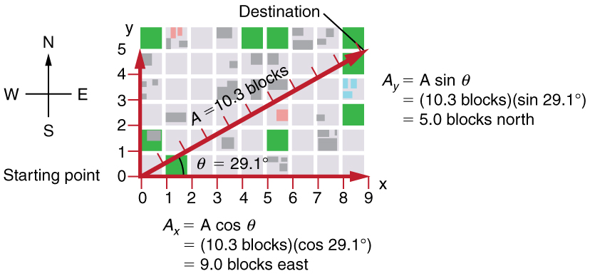
Figure 2. A person walks 9 blocks east and 5 blocks north. The displacement is 10.3 blocks at an angle  north of east.
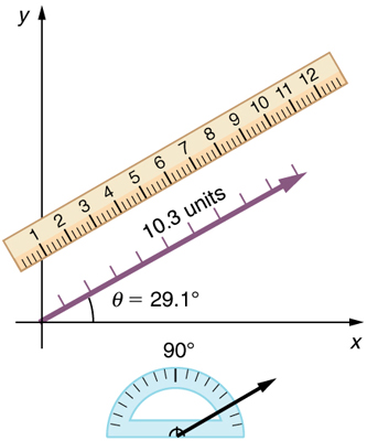
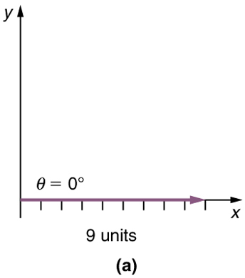
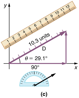
Figure 3. To describe the resultant vector for the person walking in a city as considered in Figure 2 graphically, draw an arrow to represent the total displacement vector  . Using a protractor, draw a line at an angle relative to the east-west axis. The length of the arrow is proportional to the vector’s magnitude and is measured along the line with a ruler. In this example, the magnitude of the vector is 10.3 units, and the direction is north of east.
Instructor’s Note
Taking some time to understand and practice the head-to-tail method is recommended; you’ll notice there’s a series of algorithmic steps, so you just need to learn the process, and it will work for any two vectors.
Vector Addition: Head-to-Tail Method
The head-to-tail method is a graphical way to add vectors, described in Figure 4 below and in the steps following. The tail[/pb_glossary] of the vector is the starting point of the vector, and the head (or tip) of a vector is the final, pointed end of the arrow.
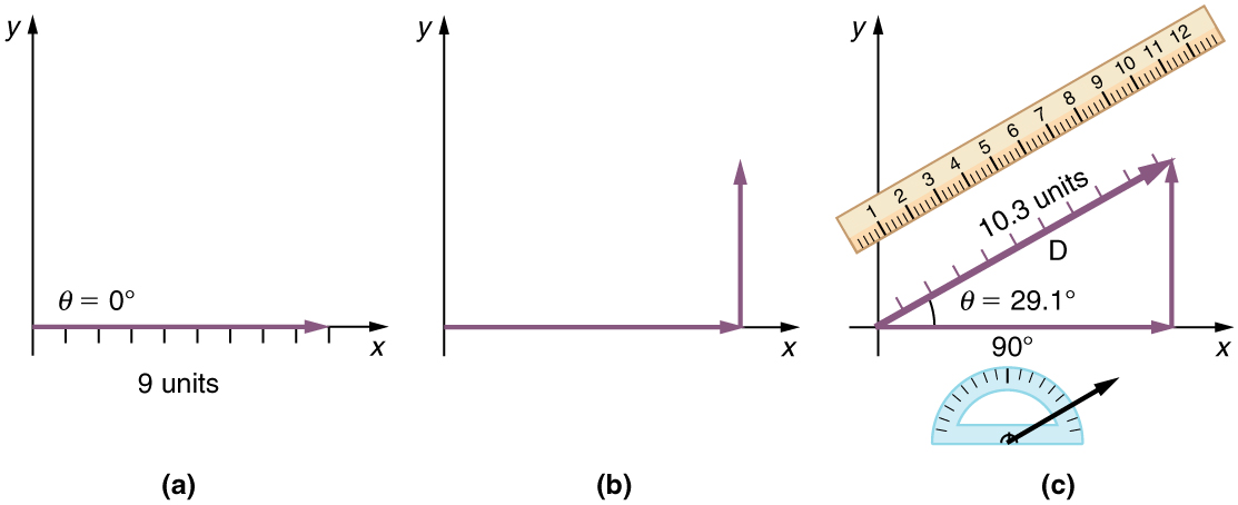 . The length of the arrow is proportional to the vector’s magnitude and is measured to be 10.3 units. Its direction, described as the angle with respect to the east (or horizontal axis) is measured with a protractor to be .
Step 1. Draw an arrow to represent the first vector (9 blocks to the east) using a ruler and protractor.
Step 2. Now draw an arrow to represent the second vector (5 blocks to the north). Place the tail of the second vector at the head of the first vector.
Step 3. If there are more than two vectors, continue this process for each vector to be added. Note that in our example, we have only two vectors, so we have finished placing the arrows tip to tail.
Step 4. Draw an arrow from the tail of the first vector to the head of the last vector. This is the resultant, or the sum, of the other vectors.
Step 5. To get the magnitude of the resultant, measure its length with a ruler. (Note that in most calculations, we will use the Pythagorean theorem to determine this length.)
Step 6. To get the direction of the resultant, measure the angle it makes with the reference frame using a protractor. (Note that in most calculations, we will use trigonometric relationships to determine this angle.)
The graphical addition of vectors is limited in accuracy only by the precision with which the drawings can be made and the precision of the measuring tools. It is valid for any number of vectors.
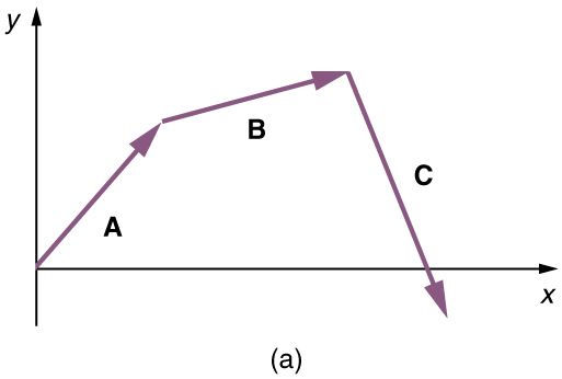
Adding Vectors Graphically using the Head-to-Tail Method: A Woman Takes a Walk
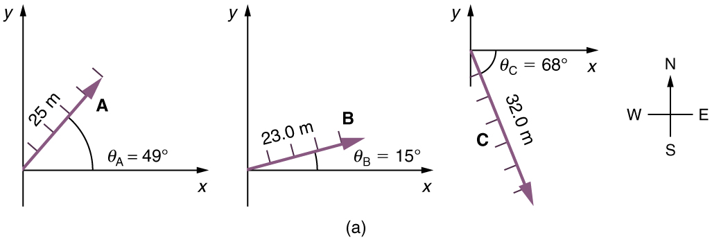
Use the graphical technique for adding vectors to find the total displacement of a person who walks the following three paths (displacements) on a flat field. First, she walks 25.0 m in a direction  north of east. Then, she walks 23.0 m heading
 north of east. Finally, she turns and walks 32.0 m in a direction
  south of east.
Strategy
Represent each displacement vector graphically with an arrow, labeling the first  , the second
  , and the third
  , making the lengths proportional to the distance and the directions as specified relative to an east-west line. The head-to-tail method outlined above will give a way to determine the magnitude and direction of the resultant displacement, denoted
Solution
(1) Draw the three displacement vectors.
(2) Place the vectors head to tail, retaining both their initial magnitude and direction.
(3) Draw the resultant vector,
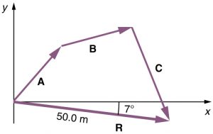
(4) Use a ruler to measure the magnitude of , and a protractor to measure the direction of . Although the direction of the vector can be specified in many ways, the easiest way is to measure the angle between the vector and the nearest horizontal or vertical axis. Because the resultant vector is south of the eastward pointing axis, we flip the protractor upside down and measure the angle between the eastward axis and the vector.
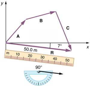
In this case, the total displacement is seen to have a magnitude of 50.0 m and to lie in a direction  south of east. By using its magnitude and direction, this vector can be expressed as
  meters and
  south of east.
Discussion
The head-to-tail graphical method of vector addition works for any number of vectors. It is also important to note that the resultant is independent of the order in which the vectors are added. Therefore, we could add the vectors in any order, as illustrated in Figure 12, and we will still get the same solution.
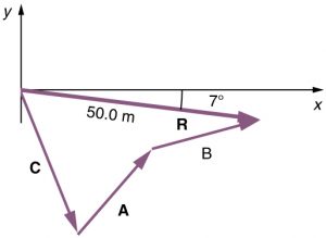
Here, we see that when the same vectors are added in a different order, the result is the same. This characteristic is true in every case and is an important characteristic of vectors. Vector addition is . Vectors can be added in any order.

(This is true for the addition of ordinary numbers as well—you get the same result whether you add  or
or  for example).
Play with Vectors
In the simulation below, choose “Explore 2-D,” and you can then
- Move vectors
 ,
,  , and
, and  on to the grid
 - Change their magnitude and direction by clicking on the tip and dragging it around.
- Manipulate the actual size using the values at the top.
- Turn on using the menus on the right:
- The components
- Angles
- Values
- Have the simulation draw the sum for you, checking the tip-to-tail method.
Vector Subtraction
Instructor’s Note
Understanding vector subtraction is necessary to understand other physics ideas. For example, acceleration is  , and
, and  is
is  . Velocity is a vector, so you’re looking at a vector subtraction whenever you’re working with acceleration.
Vector subtraction is a straightforward extension of vector addition. To define subtraction (say we want to subtract from, written  , we must first define what we mean by subtraction. The negative of a vector is defined to be
  ; that is, graphically the negative of any vector has the same magnitude but the opposite direction, as shown in Figure 13. In other words, has the same length as , but points in the opposite direction. Essentially, we just flip the vector so it points in the opposite direction.
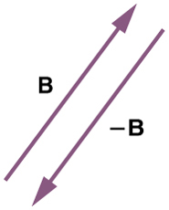 is the negative of ; it has the same length but opposite direction.
The subtraction of vector from vector is then simply defined to be the addition of to . Note that vector subtraction is the addition of a negative vector. The order of subtraction does not affect the results.
 .
.
This is analogous to the subtraction of scalars (where, for example,  . Again, the result is independent of the order in which the subtraction is made. When vectors are subtracted graphically, the techniques outlined above are used, as the following example illustrates.
Subtracting Vectors Graphically: A Woman Sailing a Boat
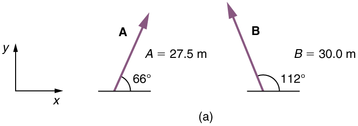
A woman sailing a boat at night is following directions to a dock. The instructions read to first sail 27.5 m in a direction  north of east from her current location, and then travel 30.0 m in a direction
  north of east (or
  west of north). If the woman makes a mistake and travels in the opposite direction for the second leg of the trip, where will she end up? Compare this location with the location of the dock.
Strategy
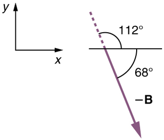
We can represent the first leg of the trip with a vector , and the second leg of the trip with a vector . The dock is located at a location  . If the woman mistakenly travels in the opposite direction for the second leg of the journey, she will travel a distance (30.0 m) in the direction
  south of east. We represent this as , as shown below. The vector has the same magnitude as but is in the opposite direction. Thus, she will end up at a location
  or .
or .
We will perform vector addition to compare the location of the dock, , with the location at which the woman mistakenly arrives, .
Solution
(1) To determine the location at which the woman arrives by accident, draw vectors and .
(2) Place the vectors head to tail.
(3) Draw the resultant vector .
(4) Use a ruler and protractor to measure the magnitude and direction of .
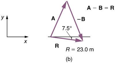
In this case,  and
and  south of east.
(5) To determine the location of the dock, we repeat this method to add vectorsand . We obtain the resultant vector  :
:
In this case  and
and  north of east.
We can see that the woman will end up a significant distance from the dock if she travels in the opposite direction for the second leg of the trip.
Discussion
Because subtraction of a vector is the same as addition of a vector with the opposite direction, the graphical method of subtracting vectors works the same as for addition.
Instructor’s Note
If you’ve taken another physics course, you’ve probably seen  . This equation will play a significant role in this class, and you’ll notice that mass is a scalar, and acceleration is a vector, so understanding how scalars and vectors multiply will be important.
Multiplication of Vectors and Scalars
If we decided to walk three times as far on the first leg of the trip considered in the preceding example, then we would walk  or 82.5 m, in a direction
  north of east. This is an example of multiplying a vector by a positive . Notice that the magnitude changes, but the direction stays the same.
If the scalar is negative, then multiplying a vector by it changes the vector’s magnitude and gives the new vector the opposite direction. For example, if you multiply by –2, the magnitude doubles but the direction changes. We can summarize these rules in the following way: When vector is multiplied by a scalar  ,
,
- The magnitude of the vector becomes the absolute value of

- If is positive, the direction of the vector does not change
- If is negative, the direction is reversed.
In our case,  and
and  . Vectors are multiplied by scalars in many situations. Note that division is the inverse of multiplication. For example, dividing by 2 is the same as multiplying by the value
  . The rules for multiplication of vectors by scalars are the same for division; simply treat the divisor as a scalar between 0 and 1.
Instructor’s Note
When dealing with vectors using analytic methods (which is covered in the next section), you need to break down vectors into essentially x-components and y-components. This next part covers this idea, so try to familiarize yourself with breaking down vectors as you read.
Resolving a Vector into Components
In the examples above, we have been adding vectors to determine the resultant vector. In many cases, however, we will need to do the opposite. We will need to take a single vector and find what other vectors added together produce it. In most cases, this involves determining the perpendicular components of a single vector, for example, the x– and y-components, or the north-south and east-west components.
For example, we may know that the total displacement of a person walking in a city is 10.3 blocks in a direction  north of east and want to find out how many blocks east and north had to be walked. This method is called finding the components (or parts) of the displacement in the east and north directions, and it is the inverse of the process followed to find the total displacement. It is one example of finding the components of a vector. There are many applications in physics where this is a useful thing to do. We will see this soon in Projectile Motion, and much more when we cover forces in Dynamics: Newton’s Laws of Motion. Most of these involve finding components along perpendicular axes (such as north and east), so that right triangles are involved. The analytical techniques presented in Vector Addition and Subtraction: Analytical Methods are ideal for finding vector components.
Section Summary
- The graphical method of adding vectors and involves drawing vectors on a graph and adding them using the head-to-tail method. The resultant vector
 is defined such that
  . The magnitude and direction of are then determined with a ruler and protractor, respectively.
 - The graphical method of subtracting vector from involves adding the opposite of vector , which is defined as . In this case, A–B=A+(–B)=R. Then, the head-to-tail method of addition is followed in the usual way to obtain the resultant vector
- Addition of vectors is commutative such that

- The head-to-tail method of adding vectors involves drawing the first vector on a graph and then placing the tail of each subsequent vector at the head of the previous vector. The resultant vector is then drawn from the tail of the first vector to the head of the final vector.
- If a vector is multiplied by a scalar quantity , the magnitude of the product is given by
 . If is positive, the direction of the product points in the same direction as ; if is negative, the direction of the product points in the opposite direction as
Vector Addition and Subtraction: Analytical Methods
Instructor’s Note
- Adding vectors by components. Don’t focus too much on what it means to add vectors. Just learn the mechanics of how to do it. We will talk about the meaning in class.
Analytical methods of vector addition and subtraction employ geometry and simple trigonometry rather than the ruler and protractor of graphical methods. Part of the graphical technique is retained because vectors are still represented by arrows for easy visualization. However, analytical methods are more concise, accurate, and precise than graphical methods, which are limited by the accuracy with which a drawing can be made. Analytical methods are limited only by the accuracy and precision with which physical quantities are known.
Resolving a Vector into Perpendicular Components
Analytical techniques and right triangles go hand-in-hand in physics because (among other things) motions along perpendicular directions are independent. We very often need to separate a vector into perpendicular components. For example, given a vector like  in Figure 1, we may wish to find which two perpendicular vectors,
  and
and  , add to produce it.
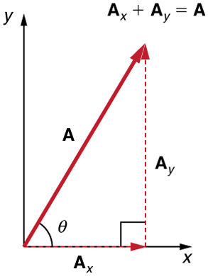
and are defined to be the components of  along the x– and y-axes. The three vectors ,
  and , form a right triangle:

Note that this relationship between vector components and the resultant vector holds only for vector quantities (which include both magnitude and direction). The relationship does not apply to the magnitudes alone. For example, if  east,
east,  north, and
  north-east, then it is true that the vectors
  . However, it is not true that the sum of the magnitudes of the vectors is also equal. That is,

Thus,

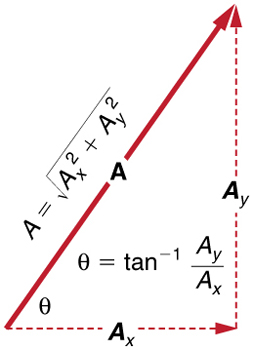
If the vector is known, then its magnitude  (its length) and its angle (its direction) are known. To find
  and
and  , its x– and y-components, we use the following relationships for a right triangle.

and
 .
.
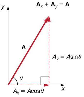 and can be related to the resultant vector and the angle with trigonometric identities. Here we see that and .
Suppose, for example, that is the vector representing the total displacement of the person walking in a city considered in Kinematics in Two Dimensions: An Introduction and Vector Addition and Subtraction: Graphical Methods.
 and to determine the magnitude of the horizontal and vertical component vectors in this example.
Then  blocks and
  , so that


Calculating a Resultant Vector
If the perpendicular components and  of a vector are known, then can also be found analytically. To find the magnitude and direction of a vector from its perpendicular components and , we use the following relationships:

 .
.
 and have been determined.
Note that the equation is just the Pythagorean theorem relating the legs of a right triangle to the length of the hypotenuse. For example, if and are 9 and 5 blocks, respectively, then  , again consistent with the example of the person walking in a city. Finally, the direction is
  , as before.
Determining Vectors and Vector Components with Analytical Methods
Equations and are used to find the perpendicular components of a vector—that is, to go from and to and . Equations and are used to find a vector from its perpendicular components—that is, to go from and to and . Both processes are crucial to analytical methods of vector addition and subtraction.
Instructor’s Note
Now that you know how to break down vectors into components, here’s a procedure for adding vectors analytically. There’s some trigonometry involved, so, again, if you’re not familiar or comfortable with trigonometry, come see your instructor. You should be familiar with both methods. You should be able to add two vectors given their x and y components, and you should be able to draw the resulting vector of the two added vectors. Also, we will go over how to use these to solve problems, so focus primarily on the methods of adding vectors.
Adding Vectors Using Analytical Methods
To see how to add vectors using perpendicular components, consider Figure 5, in which the vectors and are added to produce the resultant .
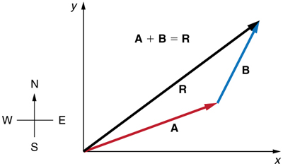 and are two legs of a walk, and is the resultant or total displacement. You can use analytical methods to determine the magnitude and direction of .
If and represent two legs of a walk (two displacements), then is the total displacement. The person taking the walk ends up at the tip of . There are many ways to arrive at the same point. In particular, the person could have walked first in the x-direction and then in the y-direction. Those paths are the x– and y-components of the resultant,  and
and  . If we know and , we can find and using the equations and . When you use the analytical method of vector addition, you can determine the components or the magnitude and direction of a vector.
Step 1. Identify the x- and y-axes that will be used in the problem. Then, find the components of each vector to be added along the chosen perpendicular axes. Use the equations and to find the components. In Figure 6, these components are , ,  and
and  . The angles that vectors and make with the x-axis are
  and
and  , respectively.
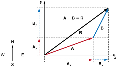 and , first determine the horizontal and vertical components of each vector. These are the dotted vectors , , and shown in the image.
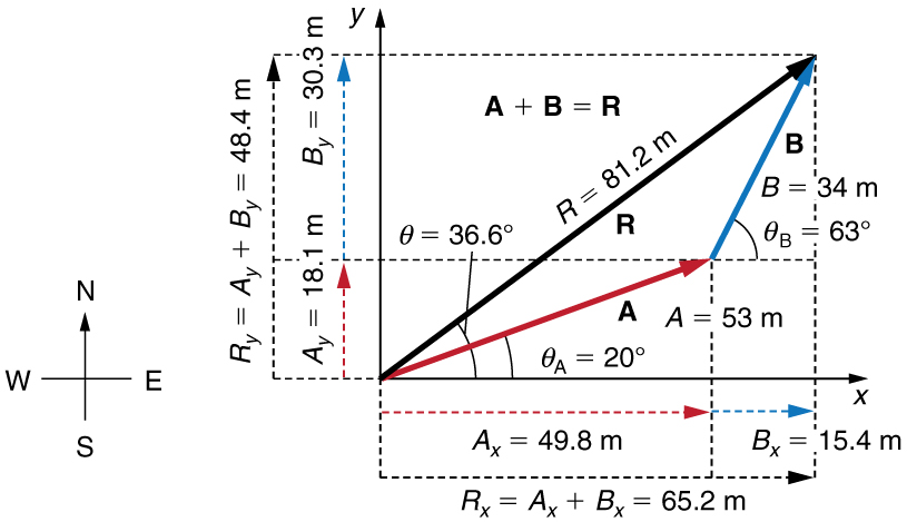
Step 2. Find the components of the resultant along each axis by adding the components of the individual vectors along that axis. That is, as shown in Figure 7,

 .
.
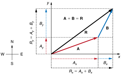 and add to give the magnitude
  of the resultant vector in the horizontal direction. Similarly, the magnitudes of the vectors and add to give the magnitude
  of the resultant vector in the vertical direction.
Components along the same axis, say the x-axis, are vectors along the same line and, thus, can be added to one another like ordinary numbers. The same is true for components along the y-axis. (For example, a 9-block eastward walk could be taken in two legs, the first 3 blocks east and the second 6 blocks east, for a total of 9, because they are along the same direction.) So, resolving vectors into components along common axes makes it easier to add them. Now that the components of are known, its magnitude and direction can be found.
Step 3. To get the magnitude  of the resultant, use the Pythagorean theorem:
Step 4. To get the direction of the resultant:
.
The following example illustrates this technique for adding vectors using perpendicular components.
Adding Vectors Using Analytical Methods
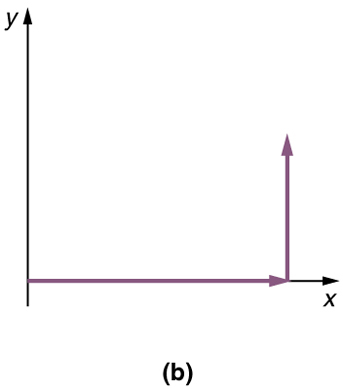
Add the vector to the vector shown in Figure 8, using perpendicular components along the x– and y-axes. The x– and y-axes are along the east–west and north–south directions, respectively. Vector represents the first leg of a walk in which a person walks  in a direction
  north of east. Vector represents the second leg, a displacement of
  in a direction
  north of east.
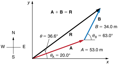 has magnitude and direction north of the x-axis. Vector has magnitude and direction north of the x-axis. You can use analytical methods to determine the magnitude and direction of .
Strategy
The components of and along the x– and y-axes represent walking due east and due north to get to the same ending point. Once found, they are combined to produce the resultant.
Solution
Following the method outlined above, we first find the components of and along the x– and y-axes. Note that  ,
,  ,
,  , and
, and  . We find the x-components by using
  , which gives:


and


Similarly, the y-components are found using  :
:


and


-components of the resultant are thus

and

Now, we can find the magnitude of the resultant by using the Pythagorean theorem:

so that

Finally, we find the direction of the resultant:

Thus,

 m and its direction is
  north of east.
Discussion
This example illustrates the addition of vectors using perpendicular components. Vector subtraction using perpendicular components is very similar—it is just the addition of a negative vector.
Subtraction of vectors is accomplished by the addition of a negative vector. That is,  . Thus, the method for the subtraction of vectors using perpendicular components is identical to that for addition. The components of are the negatives of the components of . The x– and y-components of the resultant
  are thus

and

and the rest of the method outlined above is identical to that for addition. (See Figure 10.)
Analyzing vectors using perpendicular components is very useful in many areas of physics, because perpendicular quantities are often independent of one another. The next module, Projectile Motion, is one of many in which using perpendicular components helps make the picture clear and simplifies the physics.
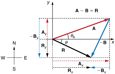 are the negatives of the components of . The method of subtraction is the same as that for addition.
More PhET Explorations: Vector Addition
This is the same simulation as above. However, now, I would recommend you look at the “Equations” option!
Section Summary
- The analytical method of vector addition and subtraction involves using the Pythagorean theorem and trigonometric identities to determine the magnitude and direction of a resultant vector.
- The steps to add vectors and
 using the analytical method are as follows:
- Determine the coordinate system for the vectors. Then, determine the horizontal and vertical components of each vector using the equations:
and
 and
and  .
. -
Add the horizontal and vertical components of each vector to determine the components
and of the resultant vector, :. - Use the Pythagorean theorem to determine the magnitude, , of the resultant vector :
 .
. - Use a trigonometric identity to determine the direction, , of :

- Determine the coordinate system for the vectors. Then, determine the horizontal and vertical components of each vector using the equations:
Homework Problems
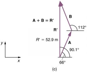
Problem 4: Find the magnitudes of the forces F1 and F2 and that add to give the total force Ftotal shown above. This may be done either graphically or by using trigonometry.
Problem 5: Suppose you walk 17.0 m straight west and then 23.0 m straight south. How far are you from your starting point, and what is the compass direction of a line connecting your starting point to your final position?
refers to the interchangeability of order in a function; vector addition is commutative because the order in which vectors are added together does not affect the final sum
a quantity with magnitude but no direction
