
23 Electric Potential
Introduction to Potential

Instructor’s Note
By the end of this section, you should know that the electric force is conservative (i.e., there is a potential energy associated with the electric force), you should be able to define what a potential is, and you should be able to calculate potential energy from a potential.
We will begin by stating that the electric force is a conservative force, which means that an electric potential energy must exist. In one of your problems, you will explore the idea of work done by a charge moving in a uniform electric field. You will see that as the charge moves around, the work done is independent of the path the charge takes, and that the work done around a closed loop path is in fact zero. The fact that the work done around a closed loop path is indicative of the fact that the electric field must be a conservative force, which should be familiar to you from previous sections.
Because the electric force is conservative, we know that we can write down a potential energy,  for the electrical force.
Instructor’s Note
As usual, some places will use  for potential energy, but in class we will use the letter capital
We’ve actually been using the idea of electric potential energy already, throughout both this class and Physics 131. The chemical energies discussed in Physics 131 are actually electric potential energies. Similarly, the potential energies of the electrons that we discussed in Units 1 and 2, unless we stated explicitly that they were gravitational potential energies, were electric potential energies.
What is the electric potential? In the figure below, we have an electron surrounding a nucleus.
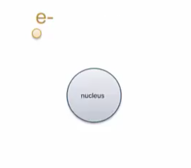
The question arises from the same place as our discussion of electrical forces: how does the electron know the nucleus is there?
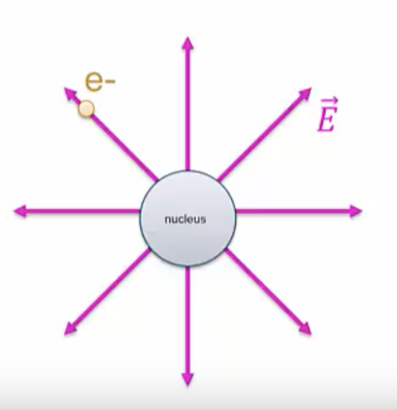
In the case of forces, we said that the nucleus generates an electric field,  . The electron is in contact with this field, and as a result feels a force,
  .
.
Essentially, we’re going to say the same thing for potential energy: the nucleus is going to generate an electric potential,  , around it. You’ll learn how to calculate these potentials from point charges in the next section. The electron does contact the potential and as a result feels a potential energy,
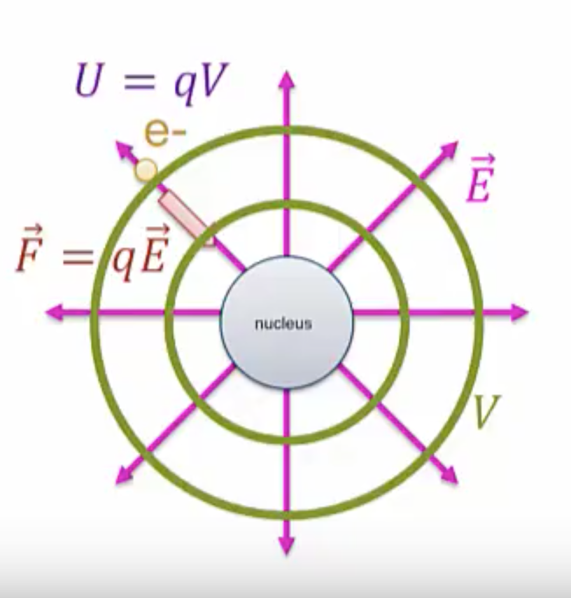
There’s a deep connection between electric field and electric potential that will be explored in a later section. Just as with electric field, the potential exists even if there is something to feel there or not, so even if we were to remove the electron, the potential would still be present.
Now let’s talk about the units of potential. The unit of potential is the Volt,  . Yes, it has the same symbol as the quantity that we’re using for potential, but we have to deal with it. One Volt is one Joule per Coulomb,
  . This definition is visible from the equation connecting potential and potential energy. If we rewrite
into
 ,
,
we know that has units of Joules,  has units of Coulombs, so, potential, is going to have units of Joules per Coulomb, which we call Volts. This second way of writing potential as
 ,
,
is why some people call potential, potential energy per unit charge. On the other hand, I want you to think of it as an invisible field around charges that gives rise to potential energy when other charged particles interact with it.
Now, let’s do an example
An electron has  of kinetic energy in a region where the potential is
  . The electron then travels to a region with a lower potential of
  .
.
What are the initial and final potential energies? What is the change in potential energy?
Solution:
Let’s begin by looking at the initial potential energy
.
We know the charge of the electron  and our initial potential is
  . So, the initial potential energy will be

Joules or converting that to electron volts, we get  .
.
Now let’s do the final potential energy, we know the charge of the electron. Again, our final potential is  . Multiplying this together, we get a final potential of

or
 .
.
Now let’s think about the change in potential energy,  . We solved for
  . Moreover, we saw our initial potential energy was
  . So the result is a change of
 .
.
Even though the potential dropped from 10V to 5V, the potential energy actually increased. This is due to the fact that the electron has a negative charge.
Instructor’s Note
Throughout our calculations, we’ve been multiplying the potential by a negative charge .
If we had instead considered a proton, then would be positive, and a positive drop in potential would result in a drop in potential energy.
Once we have changes in potential energy, we can then move on to solve problems using conservation of energy as we’ve been doing throughout this course.
One last point to discuss is the connection between the volt and the electron volt. You may have already started to see this connection in the last problem. Throughout this course and in Physics 131, we’ve been using the electron volt as a unit of energy, and we’ve just been using it as a straight conversion factor,

Now, however, you have enough information to understand where this unit of energy comes from: 1eV is the increase in energy of an electron as it goes across a 1-volt potential drop. To solve it out, we know
so the change in is the charge times the change in potential. The charge of the electron is  . A unit potential drop would be a change in potential of
  and so multiplying it all out we see that an electron going across a 1-volt potential drop has an increase in potential energy of
  which we recognize as 1eV.
Instructor’s Note
In Summary:
- Potential is to potential energy as electric field is to electric force.
- Forces result in charged objects interacting, forces result from charged particles interacting with the fields generated by other charged objects through

- Potential energies result from charged objects interacting with the potentials generated by other charged objects, mathematically written as
- Fields and potentials have the same sort of relationship as forces and potential energies.
- We can solve many problems by looking at it either in terms of fields and potentials, just like we can solve many problems by looking at it in terms of forces or potential energies.
- The unit of potential is the volt, where one volt is equal to one Joule per Coulomb, and the electron volt as a unit of energy arises from the amount of energy gained by an electron going across a one-volt potential difference.
Some Common Misconceptions About Potential
The familiar term voltage is the common name for potential difference. Keep in mind that whenever a voltage is quoted, it is understood to be the potential difference between two points. For example, every battery has two terminals, and its voltage is the potential difference between them. More fundamentally, the point you choose to be zero volts is arbitrary. This is analogous to the fact that gravitational potential energy has an arbitrary zero, such as sea level or perhaps a lecture hall floor.
In summary, the relationship between potential difference (or voltage) and electrical potential energy is given by
 .
.
Voltage is not the same as energy. Voltage is the energy per unit charge. Thus, a motorcycle battery and a car battery can both have the same voltage (more precisely, the same potential difference between battery terminals), yet one stores much more energy than the other because  . The car battery can move more charge than the motorcycle battery, although both are 12 V batteries.
Calculating Energy
Suppose you have a 12.0 V motorcycle battery that can move 5000 C of charge, and a 12.0 V car battery that can move 60,000 C of charge. How much energy does each deliver? (Assume that the numerical value of each charge is accurate to three significant figures.)
Strategy
To say we have a 12.0 V battery means that its terminals have a 12.0 V potential difference. When such a battery moves charge, it puts the charge through a potential difference of 12.0 V, and the charge is given a change in potential energy equal to  .
.
So to find the energy output, we multiply the charge moved by the potential difference.
Solution
For the motorcycle battery,  and
and  . The total energy delivered by the motorcycle battery is


 .
.
Similarly, for the car battery,  and
and

 .
.
Discussion
Although voltage and energy are related, they are not the same thing. The voltages of the batteries are identical, but the energy supplied by each is quite different. Note also that as a battery is discharged, some of its energy is used internally and its terminal voltage drops, such as when headlights dim because of a low car battery. The energy supplied by the battery is still calculated as in this example, but not all of the energy is available for external use.
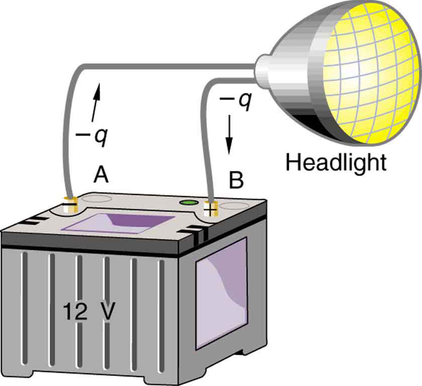
Note that the energies calculated in the previous example are absolute values. The change in potential energy for the battery is negative, because it loses energy. These batteries, like many electrical systems, actually move negative charge—electrons in particular. The batteries repel electrons from their negative terminals (A) through whatever circuitry is involved and attract them to their positive terminals (B) as shown in Figure 4. The change in potential is  and the charge is negative, so that
  is negative, meaning the potential energy of the battery has decreased when has moved from A to B.
How Many Electrons Move through a Headlight Each Second?
When a 12.0 V car battery runs a single 30.0 W headlight, how many electrons pass through it each second?
Strategy
To find the number of electrons, we must first find the charge that moved in 1.00 s. The charge moved is related to voltage and energy through the equation . A 30.0 W lamp uses 30.0 joules per second. Since the battery loses energy, we have  and, since the electrons are going from the negative terminal to the positive, we see that
  .
.
Solution
To find the charge moved, we solve the equation  :
:
 .
.
Entering the values for  and
and  , we get
 .
.
The number of electrons  is the total charge divided by the charge per electron. That is,

Discussion
This number is very large. It is no wonder that we do not ordinarily observe individual electrons with so many being present in ordinary systems. In fact, electricity had been in use for many decades before it was determined that the moving charges in many circumstances were negative. Positive charge moving in the opposite direction of negative charge often produces identical effects; this makes it difficult to determine which is moving or whether both are moving.
Problem 14: A lightning bolt strikes a tree, moving charge through a potential difference. What energy was dissipated?
Problem 15: An evacuated tube uses an accelerating voltage to accelerate electrons to hit a copper plate and produce X rays. What would be the final speed of such an electron?
Electrical Potential Due to a Point Charge
Point charges, such as electrons, are among the fundamental building blocks of matter. Furthermore, spherical charge distributions (like on a metal sphere) create external electric fields exactly like a point charge. The electric potential due to a point charge is, thus, a case we need to consider. Using calculus to find the work done by a non-conservative force to move a small charge from a large distance away, against the electric field, to a distance of  from a point charge
  , it can be shown that the electric potential of a point charge is
 ,
,
where  as usual.
As with potential energy, the potential at infinity is chosen to be zero. Thus for a positive point charge decreases with distance.
Recall that the electric potential is a scalar and has no direction, whereas the electric field  is a vector. To find the voltage due to a combination of point charges, you add the individual voltages as numbers. To find the total electric field, you must add the individual fields as vectors, taking magnitude and direction into account. This is consistent with the fact that is closely associated with energy, a scalar, whereas is closely associated with force, a vector.
What Voltage Is Produced by a Small Charge on a Metal Sphere?
Charges in static electricity are typically in the nanocoulomb  to microcoulomb
  range. What is the voltage 5.00 cm away from the center of a 1-cm diameter metal sphere that has a
  static charge?
Strategy
As we have discussed in Electric Charge and Electric Field, charge on a metal sphere spreads out uniformly and produces a field like that of a point charge located at its center. Thus, we can find the voltage using the equation  .
.
Solution
Entering known values into the expression for the potential of a point charge, we obtain

 .
.
Discussion
The negative value for voltage means a positive charge would be attracted from a larger distance, because the potential is lower (more negative) than at larger distances. Conversely, a negative charge would be repelled, as expected.
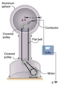
What Is the Excess Charge on a Van de Graaff Generator
A demonstration Van de Graaff generator has a 25.0 cm diameter metal sphere that produces a voltage of 100 kV near its surface. (See Figure 5.) What excess charge resides on the sphere? (Assume that each numerical value here is shown with three significant figures.)
Strategy
The potential on the surface will be the same as that of a point charge at the center of the sphere, 12.5 cm away. (The radius of the sphere is 12.5 cm.) We can thus determine the excess charge using the equation
.
Solution
Solving for and entering known values gives


 .
.
Discussion
This is a relatively small charge, but it produces a rather large voltage. We have another indication here that it is difficult to store isolated charges.
The voltages in both of these examples could be measured with a meter that compares the measured potential with ground potential. Ground potential is often taken to be zero (instead of taking the potential at infinity to be zero). It is the potential difference between two points that is of importance, and very often there is a tacit assumption that some reference point, such as Earth or a very distant point, is at zero potential, similar to the process described in Unit I – Chapter 5 Some Energy Ideas that Might Be New or Are Particularly Important. Choosing the Earth or some other reference point to be  is analogous to taking sea level as
  when considering gravitational potential energy,
  .
.
Equipotential Lines
We can represent electric potentials (voltages) pictorially, just as we drew pictures to illustrate electric fields. Of course, the two are related. Consider Figure 6, which shows an isolated positive point charge and its electric field lines. Electric field lines radiate out from a positive charge and terminate on negative charges. We use blue arrows to represent the magnitude and direction of the electric field, and we use green lines to represent places where the electric potential is constant. These are called equipotential lines in two dimensions, or equipotential surfaces in three dimensions. The term equipotential is also used as a noun, referring to an equipotential line or surface. The potential for a point charge is the same anywhere on an imaginary sphere of radius surrounding the charge. This is true because the potential for a point charge is given by  and, thus, has the same value at any point that is a given distance from the charge. An equipotential sphere is a circle in the two-dimensional view of Figure 6. Because the electric field lines point radially away from the charge, they are perpendicular to the equipotential lines.
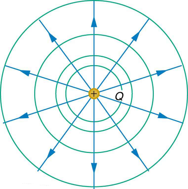 with its electric field lines in blue and equipotential lines in green. The potential is the same along each equipotential line, meaning that no work is required to move a charge anywhere along one of those lines. Work is needed to move a charge from one equipotential line to another. Equipotential lines are perpendicular to electric field lines in every case.
It is important to note that equipotential lines are always perpendicular to electric field lines. No work is required to move a charge along an equipotential, because  . Work is zero if force is perpendicular to motion. Force is in the same direction as , so that motion along an equipotential must be perpendicular to . More precisely, work is related to the electric field by
 .
.
Note that in the above equation,  and
and  symbolize the magnitudes of the electric field strength and force, respectively. Neither nor nor
  is zero, and so
  must be 0, meaning
  must be 90º. In other words, motion along an equipotential is perpendicular to .
One of the rules for static electric fields and conductors is that the electric field must be perpendicular to the surface of any conductor. This implies that a conductor is an equipotential surface in static situations. There can be no voltage difference across the surface of a conductor, or charges will flow.
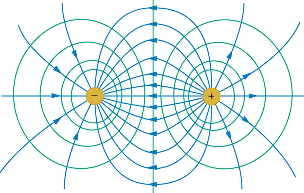
Because a conductor is an equipotential, it can replace any equipotential surface. For example, in Figure 7, a charged spherical conductor can replace the point charge, and the electric field and potential surfaces outside of it will be unchanged, confirming the contention that a spherical charge distribution is equivalent to a point charge at its center.
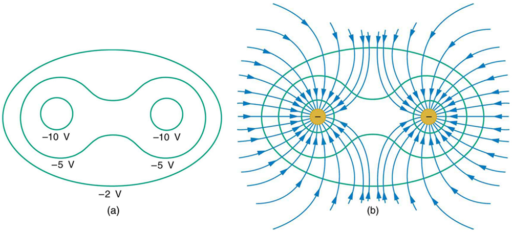
Figure 7 shows the electric field and equipotential lines for two equal and opposite charges. Given the electric field lines, the equipotential lines can be drawn simply by making them perpendicular to the electric field lines. Conversely, given the equipotential lines, as in Figure 8(a), the electric field lines can be drawn by making them perpendicular to the equipotentials, as in Figure 8(b).
Section Summary
- An equipotential line is a line along which the electric potential is constant.
- An equipotential surface is a three-dimensional version of equipotential lines.
- Equipotential lines are always perpendicular to electric field lines.
Problem 18: Electric field lines are always___________.
Problem 19: Electric field lines ____________.
The Relationship Between Electric Potential and Electric Field
We now want to explore the relationship between electric field  and electric potential
  . These ideas are simply two different ways of looking at the same phenomenon: two like-charges repel and opposite charges attract. One approach uses forces and the other uses energy. An analogous situation from Physics 131 would be the falling of a ball due to gravity: I can either think about the force of gravity
  causing the ball to accelerate down and increase speed, or I can think about the ball exchanging gravitational potential energy
  for kinetic energy
  . The final answer for the ball’s speed when it hits the ground is the same regardless of approach. In this section, we want to explore how to convert from one of these pictures to the other, and, along the way, discover a different (but equivalent) unit for electric field.
In Figure 9, we see the two approaches applied to a nucleus attracting an electron. In one picture, the nucleus generates an electric field

The electric field points away from the nucleus. The electron then interacts with that field and feels a force  . In the second picture, the nucleus generates an electric potential

which decreases from the nucleus outward. The electron then interacts with this potential by feeling a potential energy  .
.
How are these two pictures, electric fields , and electric potentials , related? Looking at the two formulas
we can see a relationship: the electric field is simply the potential divided by  ! Although there are formally some holes in this mathematical reasoning, the fundamental result is correct:

The magnitude of the electric field is the change in potential between the two points divided by the distance between those two points. This is a slope (i.e., derivative) thing like velocity or acceleration: to get the electric field at a point, you need to look at the change in potential immediately on either side and divide by the tiny distance between them. Only for uniform fields will this equation give exact results; otherwise, it gives an average electric field value.
One thing to note is that the equation indicates that the units for electric field will be Volts/meter  . However, we already know from that the units for electric field are Newtons/Coulomb
  . We are therefore forced to conclude that these two units are the same:

If we “break up” a Newton  , a Volt
  , and a Joule
  , we can see that they are the same:


(The fact that we end up with an obviously true statement of N/C = N/C means that our starting assertion that N/C = V/m was true.) Because Volts are much easier to measure and control in the lab, the units of V/m are probably more commonly used than N/C.
There is one final issue we need to address: the electric field is a vector having magnitude and direction, while the potential is a scalar, having only a magnitude. How can we determine the direction? Again, we turn to gravity for an analogy. We notice that the force of gravity points toward lower potential energy (down the hill). This is true for electricity as well: the electric field points down the “potential hill.” In the example in Figure 9 above, the electric potential from the nucleus decreases with distance, and the electric field points away from the nucleus. In general, the electric field points down the steepest slope in electric potential. We write this mathematically as

where the negative sign tells us that the electric field points down hill: from one equipotential to the next lower, always perpendicular to the equipotential lines as described in the previous section. We will practice this idea more in class.
What is the Highest Voltage Possible between Two Plates?
Dry air will support a maximum electric field strength of about  . Above that value, the field creates enough ionization in the air to make the air a conductor. This allows a discharge or spark that reduces the field. What, then, is the maximum voltage between two parallel conducting plates separated by 2.5 cm of dry air (as we will see in class, two parallel plates generate a uniform electric field)?
Strategy
We are given the maximum electric field between the plates and the distance between them. The equation  with
with  and
and  can thus be used to calculate the maximum voltage.
Solution
The potential difference or voltage between the plates is
 .
.
Entering the given values for and gives

or
 .
.
(The answer is quoted to only two digits because the maximum field strength is approximate.)
Discussion
One of the implications of this result is that it takes about 75 kV to make a spark jump across a 2.5 cm (1 in.) gap, or 150 kV for a 5 cm spark. This limits the voltages that can exist between conductors, perhaps on a power transmission line. A smaller voltage will cause a spark if there are points on the surface, because points create greater fields than smooth surfaces. Humid air breaks down at a lower field strength, meaning that a smaller voltage will make a spark jump through humid air. The largest voltages can be built up, say with static electricity, on dry days.
Field and Force inside an Electron Gun
(a) An electron gun has parallel plates separated by 4.00 cm and gives electrons 25.0 keV of energy. What is the electric field strength between the plates? (b) What force would this field exert on a piece of plastic with a  charge that gets between the plates?
Strategy
The voltage and plate separation are given, so the electric field strength can be calculated directly from the expression  . Once the electric field strength is known, the force on a charge is found using
  . Because the electric field is in only one direction, we can write this equation in terms of the magnitudes, .
Solution for (a)
The expression for the magnitude of the electric field between two uniform metal plates is
.
The electron is a single charge and is given 25.0 keV of energy, so the potential difference must be 25.0 kV. Entering this value for  and the plate separation of 0.0400 m, we obtain
 .
.
Solution for (b)
The magnitude of the force on a charge in an electric field is obtained from the equation
Substituting known values gives
 .
.
Discussion
Note that the units are newtons, because  . The force on the charge is the same no matter where the charge is located between the plates. This is because the electric field is uniform between the plates.
Problem 20: Which of the following are units of electric field?
Problem 21: Membrane walls of living cells have surprisingly large electric fields across them due to separation of ions. What is the voltage across an 8.00 nm thick membrane if the electric field strength across it is 5.25 MV/m? You may assume a uniform electric field.
Problem 22: The electric field strength between two parallel conducting plates separated by 6.4 cm is 7.0 ×10⁴ V/m. What is the potential difference between the plates given the electric field and separation? The plate with the lowest potential is taken to be at zero volts. What is the potential 1.0 cm from that plate?
Problem 23: Find the maximum potential difference between two parallel conducting plates separated by 0.55 cm of air, given the maximum sustainable electric field strength in air to be 3.00 MV/m.
A PhET to Explore These Ideas
A few things to play around with in the simulation above:
1. Add a positive and negative charge with about 5 cm of space between them. Describe what the electric field looks like.
2. Use the device to plot equipotential lines (locations where the electric potential is the same). Describe what the equipotentials look like.
3. Is there a relationship between the electric field and the equipotentials?
4. What happens if you add more charges?
