Appendix W: Absolute References

Let’s add a percent of total calculation to to Column B beginning in cell B3. The percent of total calculation shows the percentage for each value in the Annual Spend column with respect to the total in cell D12. However, after the formula is created, it will be necessary to turn off Excel’s relative referencing feature before copying and pasting the formula to the rest of the cell locations in the column. Turning off Excel’s relative referencing feature is accomplished through an absolute reference. The following steps explain how this is done:

1. Click cell B3 in the Budget Detail worksheet.
2. Type an equal sign =.
3. Click cell D3.
4. Type a forward slash /.
5. Click cell D12.
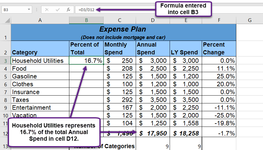
6. Press the ENTER key. You will see that Household Utilities represents 14.23% of the Annual Spend budget (see Figure 4.4).

Figure 4.4 shows the completed formula that is calculating the percentage that Household Utilities Annual Spend represents to the total Annual Spend for the budget (see cell B3). Normally, we would copy this formula and paste it into the range B4:B11. However, because of relative referencing, both cell references will increase by one row as the formula is pasted into the cells below B3. This is fine for the first cell reference in the formula (D3) but not for the second cell reference (D12).

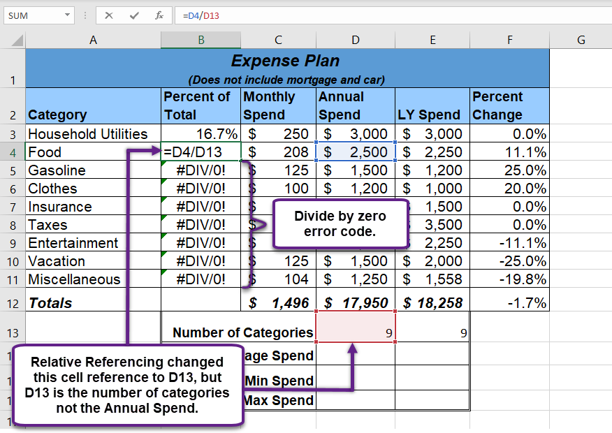
Figure 4.5 illustrates what happens if we paste the formula into the range B4:B12 in its current state. Notice that Excel produces the #DIV/0 error code. This means that Excel is trying to divide a number by zero, which is impossible. Looking at the formula in cell B4, you see that the first cell reference was changed from D3 to D4. This is fine because we now want to divide the Annual Spend for Insurance by the total Annual Spend in cell D12. However, Excel has also changed the D12 cell reference to D13. Because cell location D13 is blank, the formula produces the #DIV/0 error code.

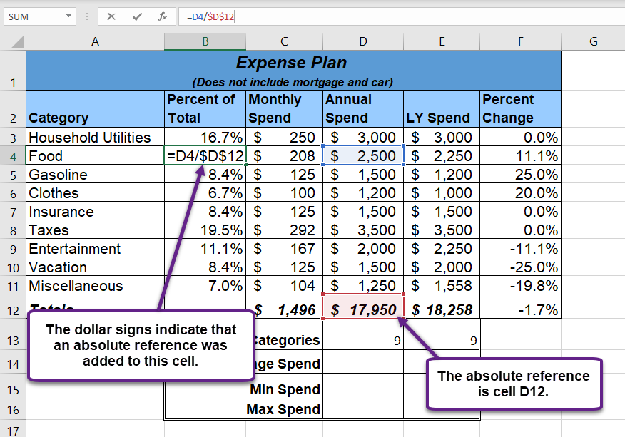
To eliminate the divide-by-zero error shown in Figure 4.5 we must add an absolute reference to cell D12 in the formula. An absolute reference prevents relative referencing from changing a cell reference in a formula. This is also referred to as locking a cell. The following explains how this is accomplished:

1. Double click cell B3.
2. Place the mouse pointer in front of D12 and click. The blinking cursor should be in front of the D in the cell reference D12.
3. Press the F4 key. You will see a dollar sign ($) added in front of the column letter D and the row number 12. You can also type the dollar signs in front of the column letter and row number.
4. Press the ENTER key.
5. Click cell B3.
6. Click the Copy button in the Home tab of the Ribbon.
7. Highlight the range B4:B11.
8. Click the Paste button in the Home tab of the Ribbon.

Figure 4.6 shows the percent of total formula with an absolute reference added to D12. Notice that in cell B4, the cell reference remains D12 instead of changing to D13 as shown in Figure 4.5. Also, you will see that the percentages are being calculated in the rest of the cells in the column, and the divide-by-zero error is now eliminated.