
5 Statistical Distributions
Brokk Toggerson
Let’s begin by looking at the distinction between a discrete and a continuous variable. Discrete variables can cannot take on any value. For example, coin tosses are either heads or tails; you can’t be half and half. Similarly, a dice will return one of the values one, two, three, four, five, or six. A dice will never return 2.342, for example. Continuous variables, on the other hand, can take on any value within a given range, and the limit of precision is not from an intrinsic limit within the system but from the measurement technique. Some examples of continuous variables include height. It is completely possible for a person to be
156.03423 centimeters tall, and we can measure a person’s height theoretically do any degree of precision that we would like.
Similarly, we often consider mass to be a continuous variable. Now, while strictly, mass is going to be discreet because you can’t have less than one electrons worth, the resolution is so small that we generally consider mass to be a continuous variable.
Now, let’s move on to thinking about probability distributions beginning with discrete data.
| Western Massachusetts County | Probability of Someone Living There |
|---|---|
| Berkshire | 0.08 |
| Franklin | 0.04 |
| Hampden | 0.29 |
| Hampshire | 0.10 |
| Worcester | 0.49 |
Here, I have a table of the probability of a given person living in one of the five western Massachusetts counties, Berkshire, Franklin, Hampton, Hampshire, and Worcester. A probability distribution is a bar graph where the height of the bar is the probability of the occurrence. So, for these data, a probability distribution would look something like this.
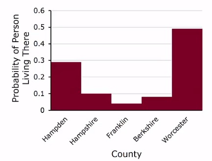
We can see each county listed on the horizontal axis, and the height of the bar indicates the probability of the person living there. All possible outcomes are in fact listed, since all possible outcomes are listed, the heights of all bars together must equal 1, because the probability of a person who lives in western mass living in one of these five counties is of course one hundred percent. Let’s think about how to use these types of graphs. So, let’s begin with this question as an example. What is the probability of a person who lives in Western Massachusetts to live in either Hampshire or Berkshire counties? We can read off the graph that the probability of a person living in Hampshire County is 10%, 0.10 while the probability of a person living in Berkshire County is a little bit less 0.08. The “or” tells us that we should add, in line with a previous video. So, the probability of a person living in Hampshire or Berkshire is the sum of the probability of a person living in Hampshire and the probability of a person living in Berkshire. Add these two probabilities together, and you get a probability of 0.18 or 18%. This is something that you need to be able to do.
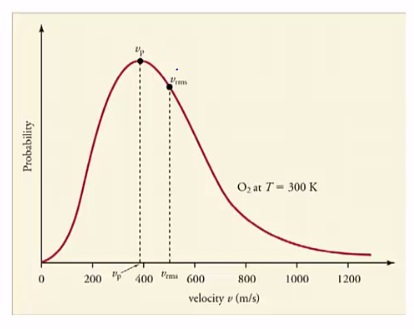
Now let’s think about probability distributions for continuous variables. Remember, continuous variables are those quantities that can take any value. An example of a continuous variable might be particle speeds at a given temperature. At a given temperature, particles have a huge variety of different speeds. The expression K= 3/2KbT tells you the average kinetic energy, or the average speed, vrms. So, let’s think about how to interpret probability distributions of continuous variables. The probability of any given number is 0. To understand this, think about what is the probability that a molecule bouncing around the room you’re
sitting in has exactly 400 meters per second worth of velocity, 400 meters per second to an infinitely high level of precision. Zero, it will always deviate from 400 by a little bit, Because of this, probability is only meaningful if we speak about range of values. Thus, to get the probability, we look at the area under the curve between the values we’re interested in.
For example, what is the probability that the velocity of an oxygen molecule at 300k has a velocity between 800 and 1200 meters per second?
Well, we have the probability distribution. The area we are interested in is the area between 800 and 1200.
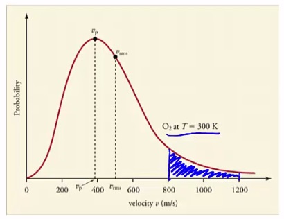
This area here tells us the probability that a given oxygen molecule has a speed within this range. Since all possible speeds are represented, the area under the entire curve will be equal to 1. The word associated with this is we say that the curve is normalized. You need to be able to recognize that probability is an area.
