Slopes and General Relationships

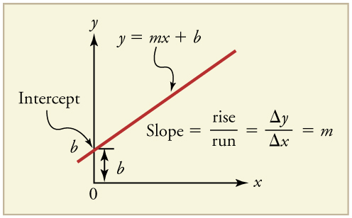
First note that graphs in this text have perpendicular axes, one horizontal and the other vertical. When two physical quantities are plotted against one another in such a graph, the horizontal axis is usually considered to be an independent variable and the vertical axis a dependent variable. If we call the horizontal axis the and the vertical axis the , as in Figure 1, a straight-line graph has the general form

Here is the slope, defined to be the rise divided by the run (as seen in the figure) of the straight line. The letter is used for the y-intercept, which is the point at which the line crosses the vertical axis.

Graph of Displacement vs. Time (a = 0, so v is constant)

Time is usually an independent variable that other quantities, such as displacement, depend upon. A graph of displacement versus time would, thus, have on the vertical axis and on the horizontal axis. Figure 2 is just such a straight-line graph. It shows a graph of displacement versus time for a jet-powered car on a very flat dry lake bed in Nevada.

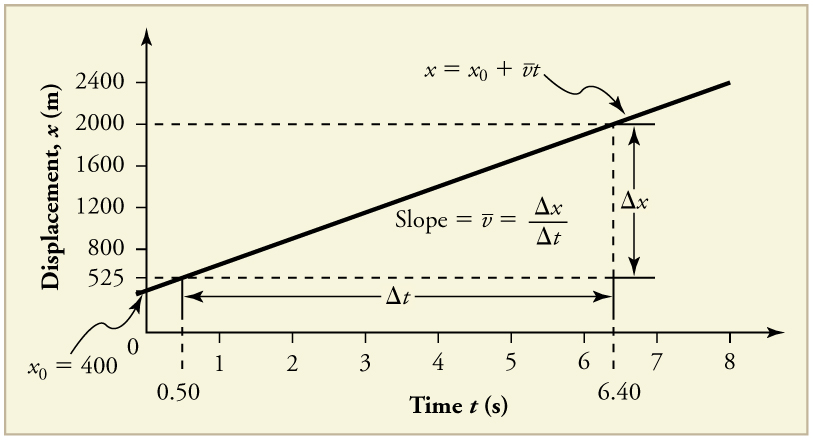
Using the relationship between dependent and independent variables, we see that the slope in the graph above is average velocity and the intercept is displacement at time zero—that is, Substituting these symbols into gives

or

Thus a graph of displacement versus time gives a general relationship among displacement, velocity, and time, as well as giving detailed numerical information about a specific situation.

From the figure we can see that the car has a displacement of 25 m at 0.50 s and 2000 m at 6.40 s. Its displacement at other times can be read from the graph; furthermore, information about its velocity and acceleration can also be obtained from the graph.

Examples: Determining Average Velocity from a Graph of Displacement versus Time: Jet Car

Problem:

Say the graph above represents the position as a function of time for a jet car. Find it’s velocity.

Solution:

The slope of a graph of vs. is velocity, since slope equals rise over run. In this case, rise = change in displacement and run = change in time, so that

Since the slope is constant here, any two points on the graph can be used to find the slope. (Generally speaking, it is most accurate to use two widely separated points on the straight line. This is because any error in reading data from the graph is proportionally smaller if the interval is larger.)

Solution

1. Choose two points on the line. In this case, we choose the points labeled on the graph: (6.4 s, 2000 m) and (0.50 s, 525 m). (Note, however, that you could choose any two points.)

2. Substitute the and values of the chosen points into the equation. Remember in calculating change we always use final value minus initial value.

,

yielding

Discussion

This is an impressively large land speed (900 km/h, or about 560 mi/h): much greater than the typical highway speed limit of 60 mi/h (27 m/s or 96 km/h), but considerably shy of the record of 343 m/s (1234 km/h or 766 mi/h) set in 1997.

Graphs of Motion when a is constant but not equal to zero

The graphs in below represent the motion of the jet-powered car as it accelerates toward its top speed, but only during the time when its acceleration is constant. Time starts at zero for this motion (as if measured with a stopwatch), and the displacement and velocity are initially 200 m and 15 m/s, respectively.

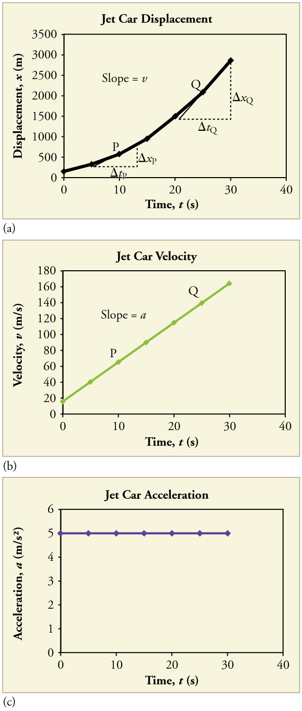
The graph of displacement versus time in sub-figure (a) is a curve rather than a straight line. The slope of the curve becomes steeper as time progresses, showing that the velocity is increasing over time. The slope at any point on a displacement-versus-time graph is the instantaneous velocity at that point. It is found by drawing a straight line tangent to the curve at the point of interest and taking the slope of this straight line. Tangent lines are shown for two points in sub-figure (a). If this is done at every point on the curve and the values are plotted against time, then the graph of velocity versus time shown in sub-figure (b) is obtained. Furthermore, the slope of the graph of velocity versus time is acceleration, which is shown in sub-figure (c).

Example: Determining Instantaneous Velocity from the Slope at a Point: Jet Car

Problem:

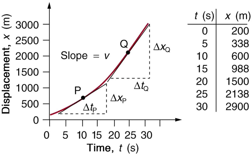
Calculate the velocity of the jet car at a time of 25 s by finding the slope of the vs. graph in the graph below.

Strategy

The slope of a curve at a point is equal to the slope of a straight line tangent to the curve at that point. This principle is illustrated in the figure above,  where Q is the point at

Solution

1. Find the tangent line to the curve at

2. Determine the endpoints of the tangent. These correspond to a position of 1300 m at time 19 s and a position of 3120 m at time 32 s.

3. Plug these endpoints into the equation to solve for the slope,

Thus,

Discussion

This is the value given in this figure’s table for at The value of 140 m/s for is plotted in the figure above. The entire graph of vs. can be obtained in this fashion.

Carrying this one step further, we note that the slope of a velocity versus time graph is acceleration. Slope is rise divided by run; on a vs. graph, rise = change in velocity and run = change in time

Key Takeaway: The slope of v vs. t

The slope of a graph of velocity vs. time is acceleration

.

Since the velocity versus time graph in the sub-figure (b) reproduced below is a straight line, its slope is the same everywhere, implying that acceleration is constant. Acceleration versus time is graphed in sub-figure (c).

Additional general information can be obtained from the figure in the prior example and the expression for a straight line,

In this case, the vertical axis is , the intercept is the slope is and the horizontal axis is Substituting these symbols yields

A general relationship for velocity, acceleration, and time has again been obtained from a graph.

It is not accidental that the same equations are obtained by graphical analysis as by algebraic techniques. In fact, an important way to discover physical relationships is to measure various physical quantities and then make graphs of one quantity against another to see if they are correlated in any way. Correlations imply physical relationships and might be shown by smooth graphs such as those above. From such graphs, mathematical relationships can sometimes be postulated. Further experiments are then performed to determine the validity of the hypothesized relationships.

Graphs of Motion Where Acceleration is Not Constant

Now consider the motion of the jet car as it goes from 165 m/s to its top velocity of 250 m/s, graphed in the figure below. Time again starts at zero, and the initial displacement and velocity are 2900 m and 165 m/s, respectively. (These were the final displacement and velocity of the car in the motion graphed above.) Acceleration gradually decreases from to zero when the car hits 250 m/s. The slope of the vs. graph increases until after which time the slope is constant. Similarly, velocity increases until 55 s and then becomes constant, since acceleration decreases to zero at 55 s and remains zero afterward.

Example: Calculating Acceleration from a Graph of Velocity versus Time

Problem:

Calculate the acceleration of the jet car at a time of 25 s by finding the slope of the vs. graph in Figure 6(b).

Strategy

The slope of the curve at is equal to the slope of the line tangent at that point, as illustrated in sub-figure (b) above.

Solution

Determine endpoints of the tangent line from the figure, and then plug them into the equation to solve for slope,

Discussion

Note that this value for is consistent with the value plotted in sub-figure (c) above at

A graph of displacement versus time can be used to generate a graph of velocity versus time, and a graph of velocity versus time can be used to generate a graph of acceleration versus time. We do this by finding the slope of the graphs at every point. If the graph is linear (i.e., a line with a constant slope), it is easy to find the slope at any point and you have the slope for every point. Graphical analysis of motion can be used to describe both specific and general characteristics of kinematics. Graphs can also be used for other topics in physics. An important aspect of exploring physical relationships is to graph them and look for underlying relationships.