7.2 Discharging Capacitor

David J. McLaughlin

7.2 Discharging Capacitor

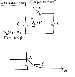
Considering a circuit comprising an initially-charged capacitor connected to a resistor through a switch as shown. The capacitor has an initial voltage $V_0$ , and the switch is open for time $t<0$ . At time $t=0$ , the switch is closed so that the capacitor discharges through the resistor. Our objective is to determine the voltage across the capacitor as a function of time, $v_c(t)$ . We will see that our circuit analysis tools (eg, KCL, KVL, Ohm’s law, the V-I relationships for the capacitor, etc…) lead to a first order differential equation, the solution of which will be $v_c(t)$ . Before beginning circuit analysis, it can be helpful to speculate what $v_c(t)$ might look like as a function of time. For $t<0$ , we know that $v_c(t)=V_0$ ; closing the switch at $t=0$ allows current to flow in the circuit, as charge and stored energy from the capacitor are released and dissipated as heat in the resistor. The capacitor voltage decreases or decays with time, eventually hitting zero as all the energy is depleted. As we shall see, the result is an exponential decay that asymptotically approaches zero.

Figure 7.1 RC discharging circuit for t<0 (upper circuit) and t>=0 (lower circuit)

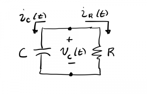
Applying KCL at the top node shown, and taking note of the fact that $v_c(t)$ is the voltage across both $R$ and $C$ , as they are connected in parallel, we have

(1) $\begin{equation*} i_{C}(t) + i_{R}(t)= 0\end{equation*}$

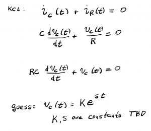
Applying the I-V relationships between current and voltage for the capacitor and the resistor, $i_C(t)=C\frac{dv_c(t)}{dt}$ and $i_R(t)=\frac{v_C(t)}{R}$ results in the differential equation

(2) $\begin{equation*} C\frac{dv_c(t)}{dt} +\frac{v_c(t)}{R}=0\end{equation*}$

which, after simple algebraic manipulation is

(3) $\begin{equation*} RC\frac{dv_c(t)}{dt} +v_c(t)=0\end{equation*}$

Equation 3 is a linear, homogeneous, first order differential equation with constant coefficients. It is linear since all terms involving $v_C(t)$ and its derivative are raised to the first power; homogeneous since all terms not involving $v_C(t)$ are zero (ie, there is no forcing function); first-order since $v_C(t)$ appears as itself and its first derivative but no higher-order derivatives, and coefficients $R$ and $C$ are constants.

One approach for solving differential equations such as this is to make an educated guess at the form of the solution. In this case, we guess that the solution is of the form

(4) $\begin{equation*} v_C(t)=Ke^{st}\end{equation*}$

where $K$ and $s$ are unknown constants to be determined. We chose this form of solution since $e^{st}$ and its derivative differ only by a multiplicative constant, and an appropriate linear combination of these two can sum to $0$ as 3 specifies. Constants $K$ and $s$ are used to keep the solution general at this point; inserting this solution back into the differential equation allows us to begin solving for the unknown constants,

(5) $\begin{equation*} RC \frac{d}{dt}{Ke^{st}} + Ke^{st} = 0\end{equation*}$

differentiating, we have

(6) $\begin{equation*} RCKse^{st} + Ke^{st} = 0\end{equation*}$

(7) $\begin{equation*} (RCse+1)Ke^{st}= 0\end{equation*}$

This equation must be true for all values of $t$ . Therefore we determine that $RCs+1=0$ from which we determine the unknown constant, $s=-\frac{1}{RC}$ . Our solution at this point can be written as:

(8) $\begin{equation*} v_c(t) = Ke^\frac{-t}{RC} \end{equation*}$

This is the result for time $t>0$ . For time $t\ge0$ we have $v_c(t)=V_0$ .

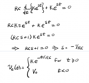
At this point, we have the solution but have a remaining constant, K, to determine. Applying the boundary condition vc(0)=Vo yields this constant.

Finally, we have the solution for vc(t) for all time, given and plotted below. While the exponential decay lasts forever, an approximate value for the duration for this transient signal is T=RC seconds.

License

Icon for the Creative Commons Attribution 4.0 International License

License

Share This Book